Estimating Slovenian Postal Areas with Voronoi Tessellation in R
From postal points to estimated areas
The interesting part of a postal code map isn’t the color fill. It’s the assumption beneath it: that each address belongs to the area around its nearest postal point. That’s how this article turns points into polygons, using Voronoi tessellation. It’s a useful way to estimate coverage, but the result depends on the points, the distance measure and the boundaries imposed on the calculation.
The method follows a project on postal codes of Spain, which provides estimated postal areas, an interactive map and GeoPackage downloads. The article now adapts that approach to Slovenia with postal points from GISCO. One difference matters immediately: Spain’s project uses CartoCiudad address points, while the Slovenian data provides one representative point for each postal code. A single point can anchor a Voronoi cell, but it says much less about how addresses are distributed across the code’s actual service area.
What a Voronoi cell represents
Take a set of shops and ask which one is closest to every location on a map. Give each shop the locations for which it is nearest, and the plane divides into regions. That partition is a Voronoi diagram, also called a Voronoi tessellation, Voronoi decomposition, Voronoi partition or Dirichlet tessellation.
Each shop is a site, or generating point. Its Voronoi cell—also known as a Thiessen polygon—contains every location at least as close to that site as to any other. Along the boundary between two cells, the two sites are equally distant. With straight-line distance, those boundaries are perpendicular bisectors between sites. Some cells continue indefinitely, so a map generally clips them to a chosen study area.
The name comes from Georgy Voronoi, who studied these partitions in the early twentieth century. The underlying idea reaches back further, including to nineteenth-century work by Dirichlet. Pokojski and Pokojska (2018) review the history and geographical uses.
Voronoi regions can help estimate which shop or public service is nearest, assign areas to weather stations, or examine spatial patterns. Thiessen polygons, for instance, can provide area weights when estimating rainfall from rain gauges. But the distance rule is doing real work here. A hospital that’s nearest as the crow flies may still be harder to reach than another one.
A small example in R
Here’s the basic geometry, stripped of geography: five points inside an imaginary square, including one at the center. The example uses sf and ggplot2; its coordinates have arbitrary units and no geographic coordinate reference system.
library(sf)
library(ggplot2)
# Define a common theme for the maps.
background <- "#faf8f2"
ink <- "#203b47"
theme_set(
theme_void() +
theme(
plot.background = element_rect(fill = background, colour = NA),
panel.background = element_rect(fill = background, colour = NA),
plot.title = element_text(face = "bold", colour = ink),
plot.subtitle = element_text(colour = ink),
plot.caption = element_text(colour = "grey40", hjust = 0),
legend.position = "bottom",
plot.margin = margin(10, 10, 10, 10)
)
)
sites <- data.frame(
site = c("A", "B", "C", "D", "E"),
x = c(2, 7, 3, 8, 5),
y = c(2, 3, 8, 7, 5)
)
toy_points <- st_as_sf(sites, coords = c("x", "y"))
study_area <- st_as_sfc(st_bbox(c(xmin = 0, ymin = 0, xmax = 10, ymax = 10)))
toy_cells <- toy_points |>
st_union() |>
st_voronoi(envelope = study_area) |>
st_collection_extract("POLYGON") |>
st_intersection(study_area)
ggplot() +
geom_sf(
data = toy_cells,
fill = c("#a8dadc", "#f4c89a", "#c6b8df", "#bfd59b", "#f2b5c4"),
colour = "white", linewidth = 1
) +
geom_sf(data = toy_points, colour = "#203b47", size = 3) +
geom_text(
data = sites, aes(x, y, label = site),
nudge_y = 0.5, colour = "#203b47", fontface = "bold"
) +
coord_sf(datum = NA) +
labs(
title = "Five points, five Voronoi cells",
subtitle = "Each location belongs to the closest site"
)
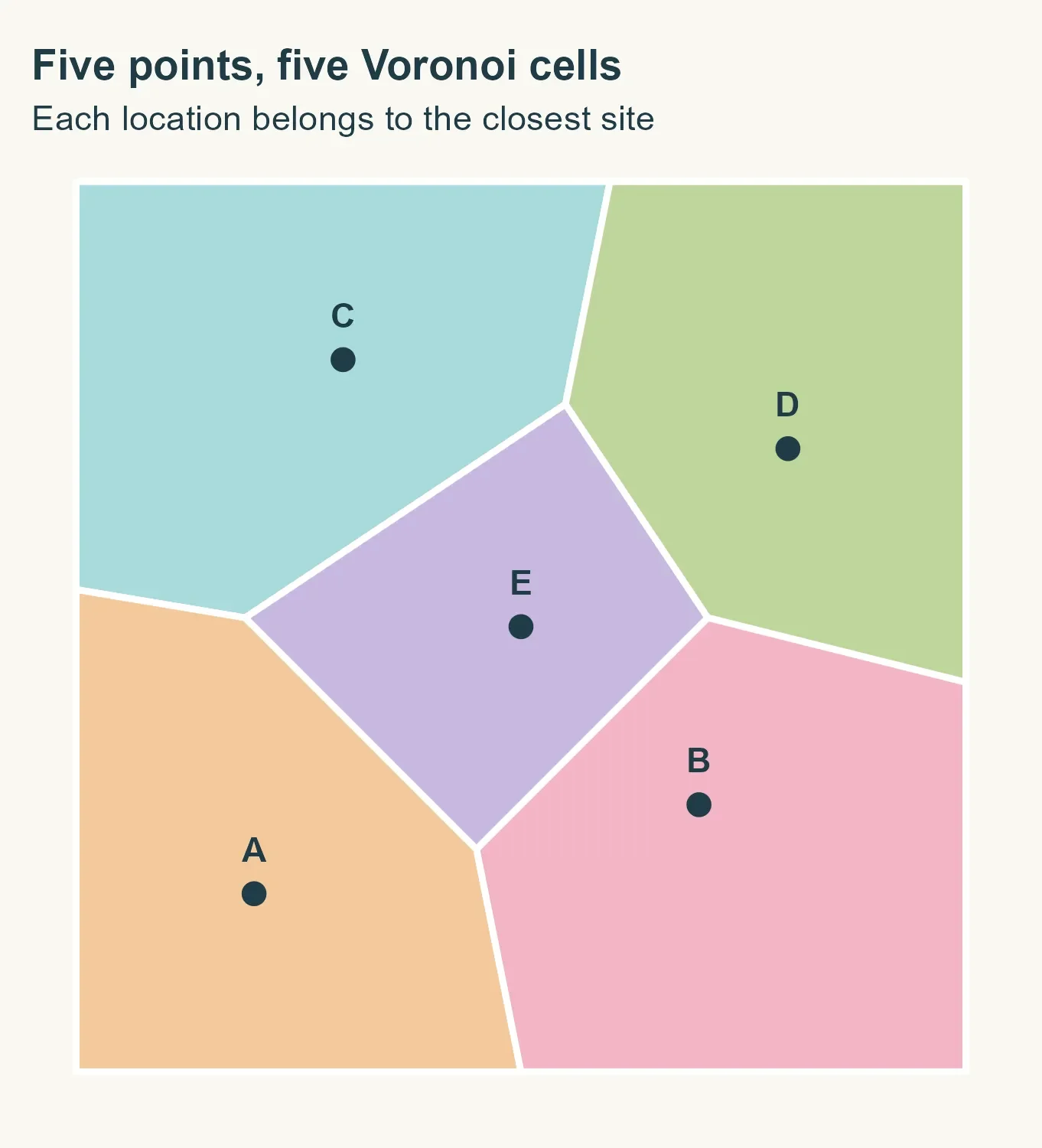
The center point E, at (5, 5), gets a bounded cell enclosed by the other four points’ regions. The outer cells run beyond the square, so the example intersects them with the square’s boundary. In the code, st_union() combines the points, st_voronoi() constructs the cells, and st_intersection() clips them. The colors simply make the regions easier to distinguish. No postal codes have been attached.
That last distinction matters. The geometry knows about point locations; it knows nothing about roads, rivers or municipal borders. Applying it to postal data means deciding explicitly which boundaries the estimate should respect.
What the Slovenian data can support
The Spanish project draws on CartoCiudad address points carrying postal codes. Its method builds on Goerlich (2022), who develops an idea presented by Sánchez (2020). The updated online version gives the method in detail.
For Slovenia, the workflow uses postal points from GISCO, retrieved with giscoR. A representative point per code is a much thinner basis for drawing boundaries than thousands of individually coded addresses. The resulting cells reflect proximity among those representatives; they can’t, by themselves, reproduce how postal delivery is organized.
There’s another assumption to keep in view: the exercise constrains estimated postal areas using municipal boundaries. The article hasn’t established that Slovenia’s postal areas follow those borders. That constraint is a modeling choice inspired by the Spanish workflow, not a verified feature of the Slovenian postal system.
This post explains the workflow. The polygons are not official postal boundaries, and the exercise does not validate the GISCO postal data.
Preparing the 2024 data
The first step downloads Slovenia’s 2024 municipal boundaries and postal points. The analysis uses ETRS89 / LAEA Europe, or EPSG:3035, a projected coordinate system measured in meters. That makes the later 200 m and 50 m buffers interpretable as distances on the map, though Voronoi still uses straight-line distances rather than travel distances, and the projection doesn’t preserve every distance exactly.
library(giscoR)
library(sf)
library(dplyr)
municipalities <- gisco_get_lau(
year = 2024, country = "SI", epsg = 3035
) |>
select(GISCO_ID, LAU_NAME) |>
st_make_valid()
raw_points <- gisco_get_postalcodes(
year = 2024, country = "SI", epsg = 3035
)
After trimming postal-code text and excluding missing or empty values, the downloaded data contains 212 municipalities and 557 postal points. All 557 points have a code, yielding 557 distinct codes, each represented by one point.
postal_points <- raw_points |>
mutate(POSTCODE = trimws(as.character(POSTCODE))) |>
filter(!is.na(POSTCODE), POSTCODE != "") |>
select(POSTCODE)
code_counts <- postal_points |>
st_drop_geometry() |>
count(POSTCODE, name = "points_per_code")
knitr::kable(data.frame(
Indicator = c(
"Municipalities", "Downloaded points", "Points with a postal code",
"Distinct postal codes", "Codes represented by one point"
),
Value = c(
nrow(municipalities), nrow(raw_points), nrow(postal_points),
nrow(code_counts), sum(code_counts$points_per_code == 1)
)
))
| Indicator | Value |
|---|---|
| Municipalities | 212 |
| Downloaded points | 557 |
| Points with a postal code | 557 |
| Distinct postal codes | 557 |
| Codes represented by one point | 557 |
Those counts describe the file; they don’t show that every Slovenian code is included or that each coordinate is correct. And with one point per code, the map will estimate regions around representative locations rather than infer them from address-level evidence.
Coincident points pose a separate problem: two points at identical coordinates can’t produce separate Voronoi cells. The workflow sorts by postal code and keeps the first record at each location. That makes the choice repeatable, but doesn’t establish that the retained code is the right one. In this dataset, it removes 79 duplicate locations; 16 locations have conflicting codes.
postal_points <- postal_points |> arrange(POSTCODE)
conflicts <- postal_points |>
group_by(geometry) |>
summarise(codes = n_distinct(POSTCODE), .groups = "drop") |>
filter(codes > 1)
duplicates <- duplicated(postal_points$geometry)
knitr::kable(data.frame(
Indicator = c("Duplicate locations removed", "Locations with conflicting codes"),
Value = c(sum(duplicates), nrow(conflicts))
))
| Indicator | Value |
|---|---|
| Duplicate locations removed | 79 |
| Locations with conflicting codes | 16 |
postal_points <- postal_points[!duplicates, ]
Testing the method in Ljubljana
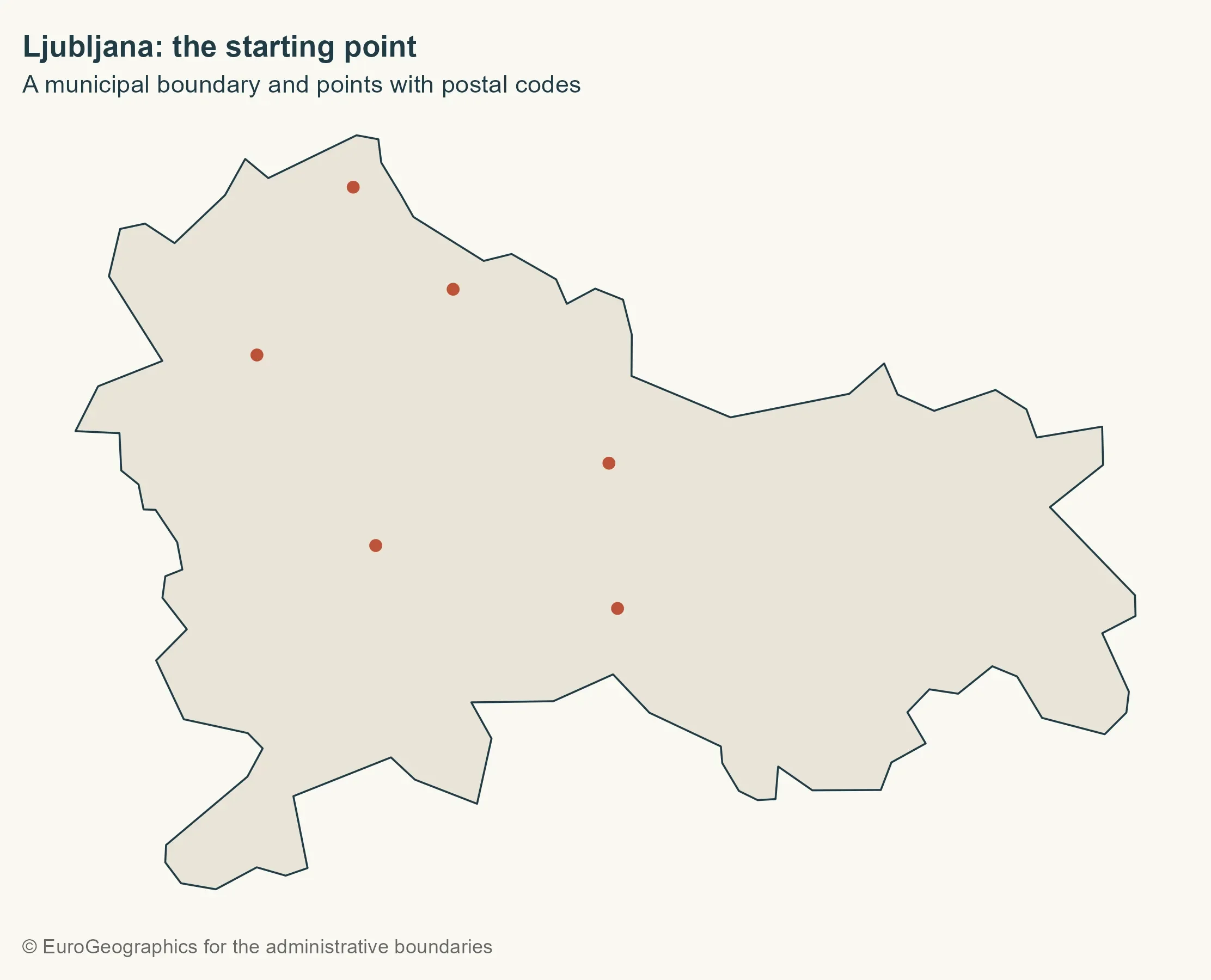
Ljubljana provides a small first case. The workflow selects points strictly within the municipality using st_within(), so a point exactly on a shared border won’t be counted in both municipalities.
city <- municipalities |> filter(LAU_NAME == "Ljubljana")
city_points <- st_filter(postal_points, city, .predicate = st_within)
base_map <- ggplot() +
geom_sf(data = city, fill = "#e8e4d8", colour = ink, linewidth = 0.4)
gisco_attr <- gisco_attributions()
base_map +
geom_sf(data = city_points, colour = "#bd5137", size = 2) +
labs(
title = "Ljubljana: the starting point",
subtitle = "A municipal boundary and points with postal codes",
caption = gisco_attr
)
Constructing and clipping the cells
For this demonstration, every interior postal point participates; the margins used later in the national workflow aren’t applied yet. The points generate Voronoi cells, using the municipality’s bounding box as the envelope.
cells <- city_points |>
st_union() |>
st_voronoi(envelope = st_as_sfc(st_bbox(city))) |>
st_collection_extract("POLYGON") |>
st_sf(geometry = _)
base_map +
geom_sf(data = cells, fill = NA, colour = "#bd5137", linewidth = 0.5) +
geom_sf(data = city_points, colour = ink, size = 2) +
labs(
title = "An area of proximity for every point",
subtitle = "Cells still extend beyond the municipal boundary",
caption = "Own elaboration using data from Eurostat / GISCO, 2024"
)
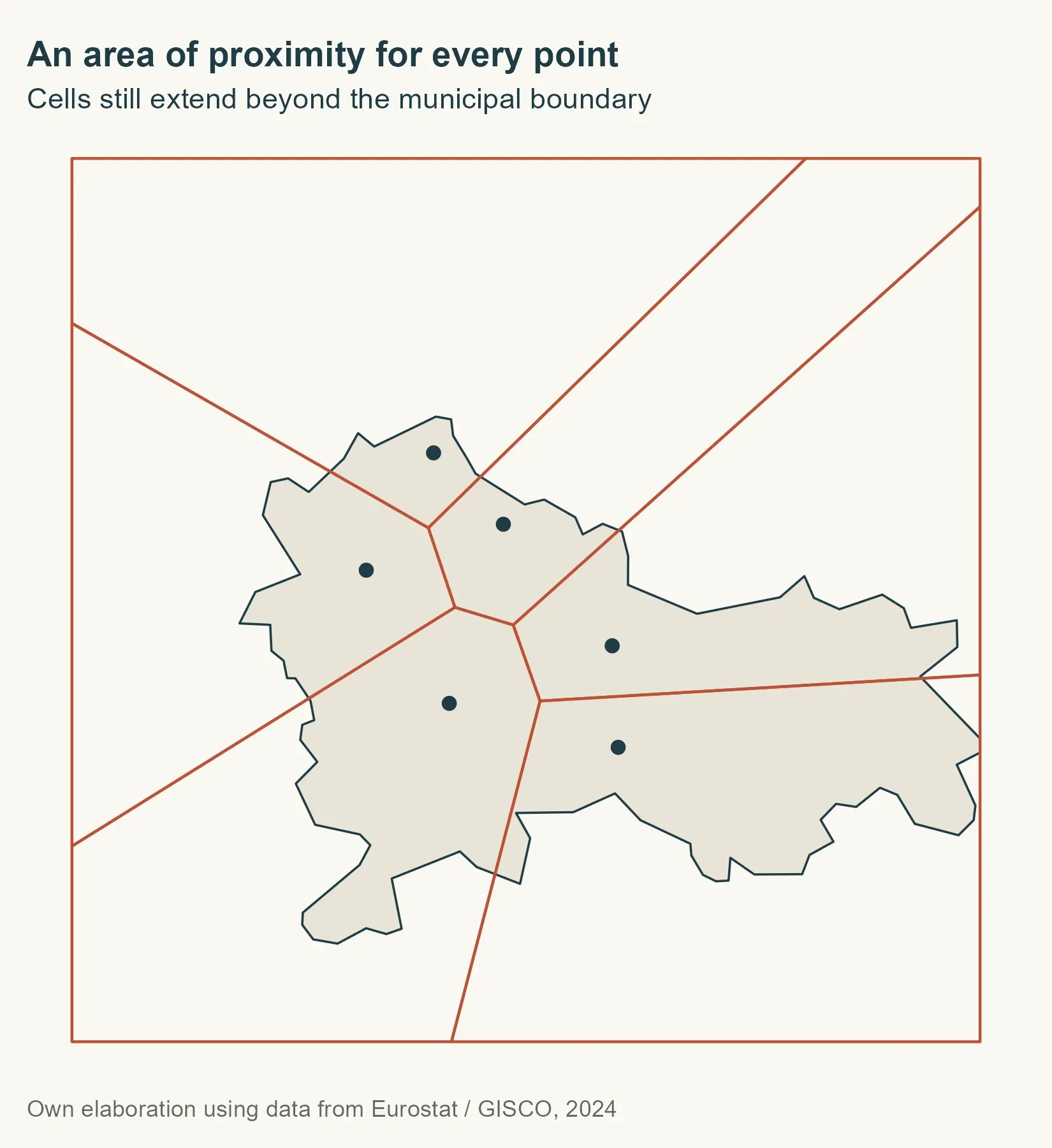
The envelope gives Voronoi a working extent; it doesn’t cut the cells to Ljubljana. That requires an explicit intersection. Cell order also shouldn’t be assumed to match input-point order, so the code finds which postal point intersects each cell and uses that relationship to attach the code. Each cell is expected to contain exactly one generating point.
point_matches <- st_intersects(cells, city_points)
cells$POSTCODE <- city_points$POSTCODE[unlist(point_matches)]
clipped_geometry <- st_intersection(st_geometry(cells), st_geometry(city))
city_cells <- st_sf(
POSTCODE = cells$POSTCODE[attr(clipped_geometry, "idx")[, 1]],
geometry = clipped_geometry
)
city_areas <- city_cells |>
group_by(POSTCODE) |>
summarise(.groups = "drop") |>
st_make_valid()
city_colours <- setNames(
hcl.colors(nrow(city_areas), palette = "Dark 3"),
sort(city_areas$POSTCODE)
)
city_labels <- st_sf(
POSTCODE = city_areas$POSTCODE,
geometry = st_point_on_surface(st_geometry(city_areas))
)
ggplot(city_areas) +
geom_sf(aes(fill = POSTCODE), colour = background, linewidth = 0.6) +
geom_sf(
data = city_points, shape = 21, fill = ink,
colour = background, size = 2.4
) +
geom_sf_text(
data = city_labels,
aes(label = POSTCODE), colour = ink, fontface = "bold", size = 3.5
) +
scale_fill_manual(values = city_colours, guide = "none") +
coord_sf(datum = NA) +
labs(
title = "From points to estimated areas",
subtitle = "Cells clipped and merged by postal code",
caption = "Teaching example · Not official postal boundaries"
)
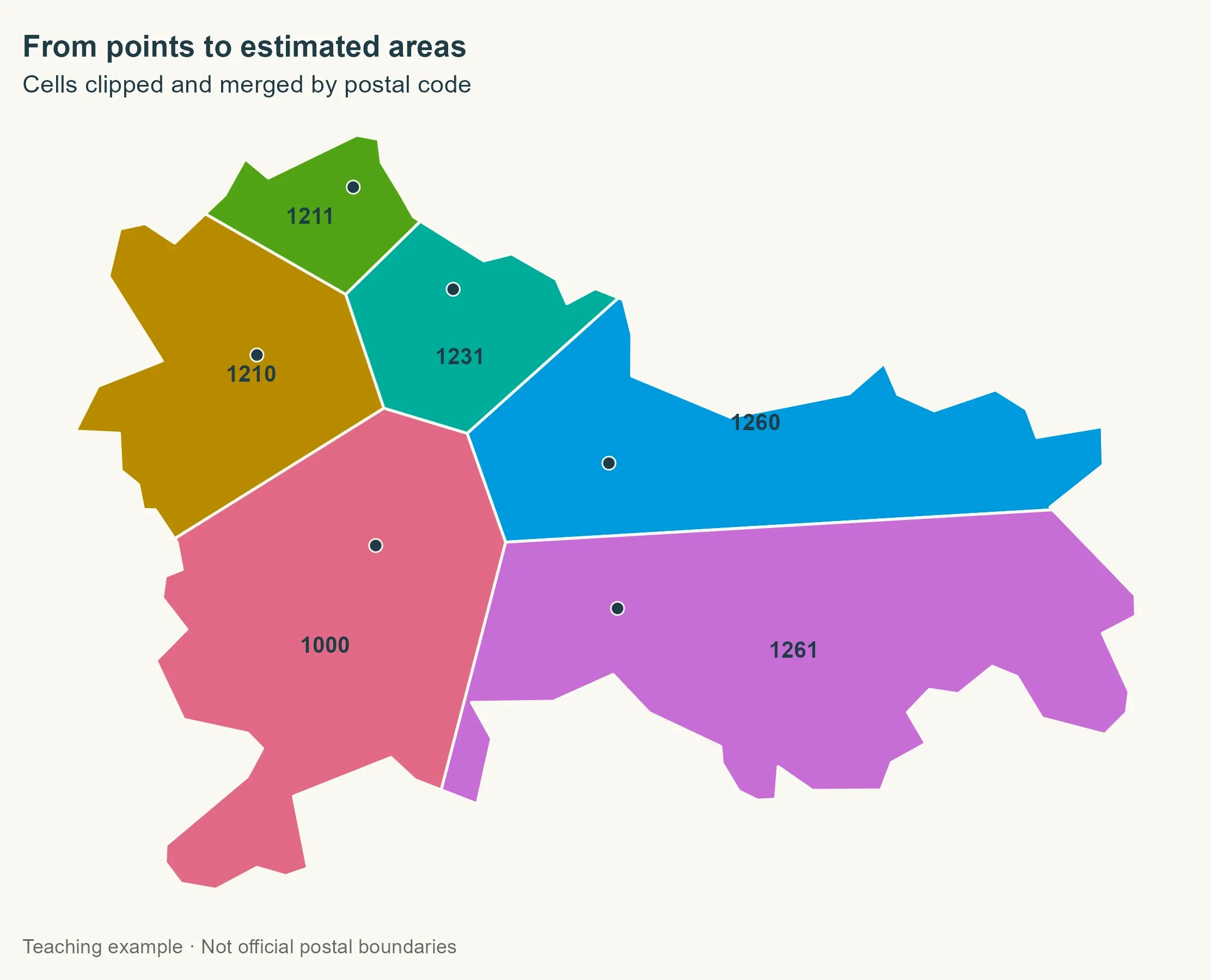
The intersection returns an index matrix that lets the workflow carry each cell’s code onto the clipped geometry. It then dissolves cells sharing a postal code. With many address points per code, that could produce one multipart geometry from several separate cells. The label locations are calculated from the area geometries themselves.
Scaling up to municipalities
For the national run, the workflow processes each polygon component of each municipality separately. Some municipalities consist of disconnected pieces; converting geometries to multipolygons and then splitting them into polygons allows each piece to be handled on its own. That avoids automatically extending a postal code into a separate component with no points. Municipality identifiers and names are marked as attributes that remain constant through the split.
components <- municipalities |>
st_set_agr("constant") |>
st_cast("MULTIPOLYGON") |>
st_cast("POLYGON") |>
mutate(component_id = row_number())
Why exclude points near borders?
The Spanish workflow first looks for addresses at least 200 m inside a municipality, then tries a 50 m inward margin if that finds none. The idea is to reduce the effect of points near borders, where small mismatches between data layers could change which side a point falls on.
Those distances aren’t universal. Goerlich describes a 20 m margin; the 200 m and 50 m settings come from this implementation. Sparse postal points make the tradeoff sharper: a large inward buffer can discard useful points. Comparing alternative margins would help show how much the estimates depend on this choice.
select_points <- function(component, postal_points) {
for (margin in c(200, 50)) {
interior <- st_buffer(st_geometry(component), -margin)
if (all(st_is_empty(interior))) next
selected_points <- st_filter(postal_points, interior,
.predicate = st_within
)
if (nrow(selected_points) > 0) {
return(selected_points)
}
}
postal_points[0, ]
}
The buffer controls which points are selected; it doesn’t shrink the final mapped area. Resulting cells are clipped to the original municipal component. If neither margin contains a point, the component remains unassigned rather than borrowing a point from outside the municipality.
Three situations in one function
The national function has three cases. A component with no selected points gets an NA postal code. If all its selected points share one code, that code covers the whole component. Voronoi construction is only needed when multiple codes are present.
build_areas <- function(component, postal_points) {
selected_points <- select_points(component, postal_points)
codes <- unique(selected_points$POSTCODE)
if (length(codes) <= 1L) {
component$POSTCODE <- if (length(codes)) codes else NA_character_
return(component)
}
cells <- selected_points |>
st_union() |>
st_voronoi(envelope = st_as_sfc(st_bbox(component))) |>
st_collection_extract("POLYGON") |>
st_sf(geometry = _)
point_matches <- st_intersects(cells, selected_points)
cells$POSTCODE <- selected_points$POSTCODE[unlist(point_matches)]
clipped_geometry <- st_intersection(
st_geometry(cells),
st_geometry(component)
)
result <- st_sf(
POSTCODE = cells$POSTCODE[attr(clipped_geometry, "idx")[, 1]],
geometry = clipped_geometry
) |>
group_by(POSTCODE) |>
summarise(.groups = "drop") |>
st_make_valid()
result$GISCO_ID <- component$GISCO_ID
result$LAU_NAME <- component$LAU_NAME
result$component_id <- component$component_id
result
}
result <- lapply(seq_len(nrow(components)), function(i) {
build_areas(components[i, ], postal_points)
}) |>
bind_rows()
Recovering some unassigned areas
A component with no points may still belong to a municipality whose other components do have postal information. The workflow fills that gap only when exactly one distinct recovered code exists elsewhere in the same municipality. It’s an imputation based on the available points, not evidence that the municipality truly has only one postal code.
unique_codes <- result |>
st_drop_geometry() |>
filter(!is.na(POSTCODE)) |>
distinct(GISCO_ID, POSTCODE) |>
add_count(GISCO_ID) |>
filter(n == 1)
unassigned_before <- sum(is.na(result$POSTCODE))
index <- match(result$GISCO_ID, unique_codes$GISCO_ID)
recoverable <- is.na(result$POSTCODE) & !is.na(index)
result$POSTCODE[recoverable] <- unique_codes$POSTCODE[index[recoverable]]
Before mapping, the workflow repairs geometries and keeps only polygon surfaces, since repairs can leave stray lines or points in geometry collections. It then dissolves by postal code, removing municipal borders wherever neighboring areas share the same code.
keep_surfaces <- function(x) {
  geometry <- st_make_valid(st_geometry(x))
  geometry <- lapply(geometry, function(part) {
    if (!inherits(part, c("POLYGON", "MULTIPOLYGON", "GEOMETRYCOLLECTION"))) {
      return(st_multipolygon())
    }
    surfaces <- suppressWarnings(st_collection_extract(st_sfc(part), "POLYGON"))
    if (length(surfaces) == 0L || all(st_is_empty(surfaces))) {
      return(st_multipolygon())
    }
    st_cast(st_union(surfaces), "MULTIPOLYGON", warn = FALSE)[[1]]
  })
  st_geometry(x) <- st_sfc(geometry, crs = st_crs(x))
  x[!st_is_empty(x), ]
}

unassigned <- result |>
  filter(is.na(POSTCODE)) |>
  keep_surfaces()

postal_areas <- result |>
  filter(!is.na(POSTCODE)) |>
  group_by(POSTCODE) |>
  summarise(.groups = "drop") |>
  keep_surfaces() |>
  st_cast("MULTIPOLYGON")
A national view, with the right caveat
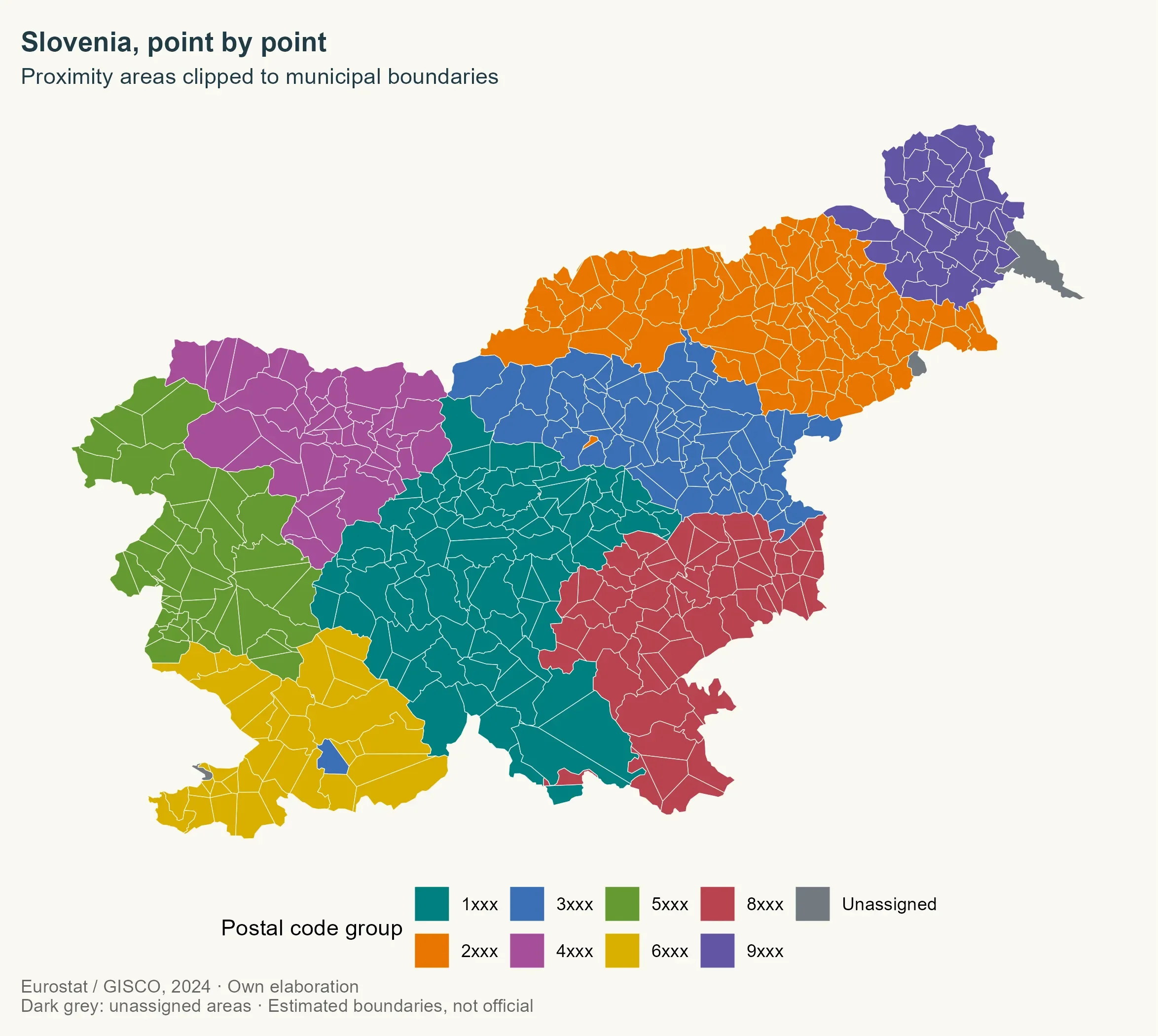
The map’s strongest feature is also its main limitation: it makes a complicated set of estimated postal areas easy to read, but the colors don’t certify that those areas match official postal regions. Grouping by the first digit gives a useful national overview while keeping the map legible. Gray marks components that remain unassigned.
postal_colours <- c(
  "1" = "#007F7F", "2" = "#E87500", "3" = "#3B6FB6", "4" = "#A64E9A",
  "5" = "#649A32", "6" = "#D9AF00", "8" = "#B94350", "9" = "#6255A4",
  "Unassigned" = "#727A80"
)

postal_groups <- sort(unique(substr(postal_areas$POSTCODE, 1, 1)))

ggplot() +
  geom_sf(data = municipalities, fill = "#d5d2ca", colour = NA) +
  geom_sf(
    data = postal_areas,
    aes(fill = substr(POSTCODE, 1, 1)), colour = background, linewidth = 0.15
  ) +
  geom_sf(
    data = unassigned, aes(fill = "Unassigned"),
    colour = background, linewidth = 0.15
  ) +
  scale_fill_manual(
    values = postal_colours, name = "Postal code group",
    breaks = c(postal_groups, "Unassigned"),
    labels = c(paste0(postal_groups, "xxx"), "Unassigned")
  ) +
  coord_sf(datum = NA) +
  labs(
    title = "Slovenia, point by point",
    subtitle = "Proximity areas clipped to municipal boundaries",
    caption = paste(
      "Eurostat / GISCO, 2024 · Own elaboration",
      "Dark grey: unassigned areas · Estimated boundaries, not official",
      sep = "\n"
    )
  )
A clean geometry is not a correct postal map
The geometry checks come back remarkably clean: the assigned and unassigned areas cover the municipal territory, and their measured overlap is effectively zero. The workflow allows a one-square-meter tolerance for small numerical discrepancies. That’s reassuring about the polygon operations, but it says nothing about whether the estimated borders reflect where postal services actually operate.
territory <- st_union(st_geometry(municipalities))
coverage <- st_union(c(st_geometry(postal_areas), st_geometry(unassigned)))

difference_m2 <- as.numeric(
  sum(st_area(st_sym_difference(territory, coverage)))
)

overlap_m2 <- as.numeric(
  sum(st_area(postal_areas)) + sum(st_area(unassigned)) - sum(st_area(coverage))
)

knitr::kable(data.frame(
  Indicator = c(
    "Codes with an estimated area", "Components assigned by municipal recovery",
    "Unassigned records", "Unassigned area (km²)",
    "Coverage difference (m²)", "Overlap (m²)"
  ),
  Value = round(c(
    nrow(postal_areas), sum(recoverable), nrow(unassigned),
    as.numeric(sum(st_area(unassigned))) / 1e6, difference_m2,
    overlap_m2
  ), 4)
))
| Indicator | Value |
|---|---|
| Codes with an estimated area | 468.0000 |
| Components assigned by municipal recovery | 4.0000 |
| Unassigned records | 6.0000 |
| Unassigned area (km²) | 150.2033 |
| Coverage difference (m²) | 0.0000 |
| Overlap (m²) | -0.0002 |
Those figures describe geometry: 468 postal codes have estimated areas, municipal recovery assigned four components, and six records remain unassigned across 150.2033 km². Coverage differs by 0.0000 m²; the calculated overlap is -0.0002 m², a tiny numerical residue. A country can be tiled perfectly by valid polygons and still have a weak postal map.
What the input points can tell you
The method runs from points to proximity areas, clips those areas to municipal boundaries, then merges them by postal code. The same sequence can use much denser address data; one example is the CartoCiudad material in my Spanish postal codes project.
Here’s the thing: the point data shapes the answer as much as the algorithm does. Give a Voronoi method one representative point per postal code and it mostly maps distances between those representatives. Give it address points and the resulting areas can better reflect where addresses cluster. Even then, the method has no information about delivery routes, physical barriers, or official postal boundaries.
There’s no independent Slovenian postal source in this analysis to validate the result against. Before using these areas for substantive analysis, you’d want to examine coverage, coordinate quality, how the estimates relate to municipalities, and how sensitive the result is to the chosen margins. For now, this is a useful demonstration of how to build the polygons, not evidence that they reproduce Slovenia’s delivery geography.
References
- Pokojski, W. & Pokojska, P. (2018). Voronoi diagrams – inventor, method, applications. Polish Cartographical Review, 50(3), 141–150. https://doi.org/10.2478/pcr-2018-0009.
- Goerlich, F. J. (2022). Elaboración de un mapa de códigos postales de España con recursos libres. Cómo evitar pagar por disponer de información de referencia. Working Papers Ivie, no. 2022-3. València: Ivie. https://doi.org/10.12842/WPIVIE_0322. Updated online version: https://www.uv.es/goerlich/Ivie/CodPost.html.
- Sánchez, J. I. (2020, November 13). “Así hice el mapa de los códigos postales de España con SIG y datos abiertos.” NoSoloSIG. https://www.nosolosig.com/articulos/asi-hice-el-mapa-de-los-codigos-postales-de-espana-con-sig-y-datos-abiertos.
- Hernangómez, D. (2026). Códigos postales de España [Dataset]. https://doi.org/10.5281/zenodo.23698418. https://dieghernan.github.io/codigospostales/.
R-bloggers.com offers daily e-mail updates about R news and tutorials about learning R and many other topics. Click here if you're looking to post or find an R/data-science job.
Want to share your content on R-bloggers? click here if you have a blog, or here if you don't.