Evaluating a U-Net Nuclei Segmentation Model Across 134 Held-Out Images
The average hides where the model struggles
In 2020, I trained a U-Net on the 2018 Data Science Bowl nuclei dataset using the first version of this package. The Dice score rose during training, and the post ended with four predicted masks on test images. Those images had no ground-truth masks, so the attractive predictions offered no way to check what the model had missed. This follow-up does that check. There’s no new training here. The model is the publisheddsbowl-unet from the first post in the series, evaluated on its held-out images. Scoring all 134 took about twelve seconds on a processor.
Rebuild the split before trusting the score
The source is BBBC038v1 from the Broad Institute: the Data Science Bowl images, released under a CC0 waiver. Itsstage1_train directory contains 670 annotated images, each in its own directory, with one mask file for each nucleus.
data_dir <- "stage1_train" # BBBC038v1, unzipped
data_dir = "stage1_train" # BBBC038v1, unzipped
split_dataset() records file lists in CSVs without copying the image files.
library(rplatypus)
split <- split_dataset(data_dir, tempfile("splits"),
fractions = c(0.8, 0.2), seed = 1)
split
#> platypus split
#> train 536 samples
#> validation 134 samples
#> every sample its own group
#> seed 1 - the same inputs give this split again
import tempfile
import pyplatypus as pp
split = pp.split_dataset(data_dir, tempfile.mkdtemp(),
fractions=(0.8, 0.2), seed=1)
split["samples"]
#> {'train': 536, 'validation': 134, 'test': 0}
stage1_validation directory containing 134 images. That matching count looks reassuring, but 101 of those images are in the training portion of the split used to measure the weights. Evaluate against that directory and the model gets credit partly for images it has already seen. The count alone won’t expose the overlap.
A strong mean, with a question attached
spec <- platypus_spec(
data = segmentation_data(split, colormap = binary_colormap),
models = list(
u_net("nuclei", input_shape = c(256, 256), blocks = 4, filters = 16,
weights = "dsbowl-unet", fit = FALSE,
metrics = list(metric_dice(include_background = FALSE)))
)
)
fit <- platypus_fit(spec, verbose = FALSE)
cases <- evaluate_cases(fit)
summary(cases)
#> metric n mean sd median min max
#> 1 dice 134 0.9205236 0.05322748 0.9313503 0.7239583 0.9860661
#> worst_case
#> 1 7f38885521586fc6011bef1314a9fb2aa1e4935bd581b2991e1d963395eab770
engine = pp.build_engine(pp.from_dict({
"task": "semantic_segmentation",
"data": {
"train_path": str(split["paths"]["train"]),
"validation_path": str(split["paths"]["validation"]),
"colormap": [[0, 0, 0], [255, 255, 255]],
"mode": "config_file",
},
"models": [{
"name": "nuclei",
"architecture": "u_net",
"input_shape": [256, 256],
"blocks": 4,
"filters": 16,
"weights": "dsbowl-unet",
"fit": False,
"metrics": [{"name": "dice", "include_background": False}],
}],
}))
engine.fit()
cases = engine.evaluate_cases("nuclei")
pp.summarise_cases(cases)
#> [{'metric': 'dice', 'n': 134, 'mean': 0.9205236150257623,
#> 'sd': 0.05322747958922138, 'median': 0.9313502907752991,
#> 'min': 0.7239583134651184, 'max': 0.9860661029815674,
#> 'worst_case':
#> '7f38885521586fc6011bef1314a9fb2aa1e4935bd581b2991e1d963395eab770'}]
include_background = FALSE. Include them and a model that detects no nuclei at all could still land around 0.5.
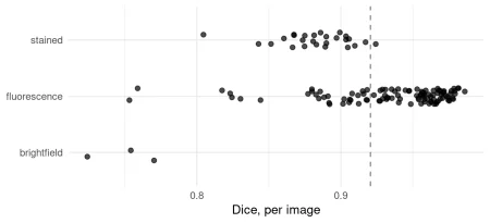
A 0.92 mean is a good result. It’s also an incomplete description. The useful question is what kinds of images make up that average.
Look at each image, then group the failures
evaluate() returns one row per model. evaluate_cases() gives one row per image, making it possible to see the cases the average smooths over.
head(cases[order(cases$dice), ], 5)
#> platypus scores by case (5 rows)
#> case dice
#> 7f38885521586fc6011bef1314a9fb2aa1e4935bd581b2991e1d963395eab770 0.7239583
#> 29ea4f6eb4545f43868a9b40a60000426bf8dfd9d062546656a37bd2a2aaf9ec 0.7531800
#> 8f94a80b95a881d0efdec36affc915dca9609f4cba8134c4a91b219d418778aa 0.7541562
#> a6515d73077866808ad4cb837ecdac33612527b8a1041e82135e40fce2bb9380 0.7588775
#> 2a1a294e21d76efd0399e4eb321b45f44f7510911acd92c988480195c5b4c812 0.7702851
worst = sorted(cases, key=lambda row: row["dice"])[:5]
[(row["case"][:16], round(row["dice"], 4)) for row in worst]
#> [('7f38885521586fc6', 0.724), ('29ea4f6eb4545f43', 0.7532),
#> ('8f94a80b95a881d0', 0.7542), ('a6515d7307786680', 0.7589),
#> ('2a1a294e21d76efd', 0.7703)]
image_kind <- function(case) {
path <- list.files(file.path(data_dir, case, "images"), full.names = TRUE)
pixels <- png::readPNG(path[1])[, , 1:3]
colour <- mean(abs(pixels[, , 1] - pixels[, , 2])) +
mean(abs(pixels[, , 2] - pixels[, , 3]))
if (colour > 0.02) return("stained")
if (mean(pixels) > 0.5) "brightfield" else "fluorescence"
}
cases$kind <- vapply(cases$case, image_kind, character(1))
aggregate(dice ~ kind, cases, function(x) {
round(c(n = length(x), mean = mean(x), min = min(x)), 3)
})
#> kind dice.n dice.mean dice.min
#> 1 brightfield 3.000 0.749 0.724
#> 2 fluorescence 105.000 0.935 0.753
#> 3 stained 26.000 0.883 0.805
from pathlib import Path
import numpy as np
from PIL import Image
def image_kind(case):
path = next((Path(data_dir) / case / "images").glob("*.png"))
pixels = np.asarray(Image.open(path).convert("RGB")) / 255
colour = (np.abs(pixels[..., 0] - pixels[..., 1]).mean()
+ np.abs(pixels[..., 1] - pixels[..., 2]).mean())
if colour > 0.02:
return "stained"
return "brightfield" if pixels.mean() > 0.5 else "fluorescence"
for row in cases:
row["kind"] = image_kind(row["case"])
kinds = sorted({row["kind"] for row in cases})
dice = {k: [r["dice"] for r in cases if r["kind"] == k] for k in kinds}
{k: (len(d), round(float(np.mean(d)), 3), round(min(d), 3))
for k, d in dice.items()}
#> {'brightfield': (3, 0.749, 0.724), 'fluorescence': (105, 0.935, 0.753),
'stained': (26, 0.883, 0.805)}
library(ggplot2)
ggplot(cases, aes(dice, kind)) +
geom_vline(xintercept = mean(cases$dice), linetype = "dashed",
colour = "grey50") +
geom_jitter(height = 0.15, width = 0, alpha = 0.7, size = 2) +
labs(x = "Dice, per image", y = NULL) +
theme_minimal(base_size = 13)
import matplotlib.pyplot as plt
rng = np.random.default_rng(1)
fig, ax = plt.subplots(figsize=(7, 3.2))
ax.axvline(np.mean([r["dice"] for r in cases]), linestyle="--", color="grey")
for i, k in enumerate(kinds):
jitter = rng.uniform(-0.15, 0.15, len(dice[k]))
ax.scatter(dice[k], i + jitter, alpha=0.7)
ax.set_yticks(range(len(kinds)), kinds)
ax.set_xlabel("Dice, per image")
predictions <- predict(fit, split = "validation")
files_of <- function(case, what) {
list.files(file.path(data_dir, case, what), full.names = TRUE)
}
truth_of <- function(case) {
masks <- lapply(files_of(case, "masks"), function(f) {
read_masks(f, binary_colormap, size = c(256, 256))[1, , ]
})
unite_masks(masks)
}
middle <- which.min(abs(cases$dice - median(cases$dice)))
shown <- c(which(cases$kind == "brightfield"), middle)
images <- read_images(
vapply(cases$case[shown], function(k) files_of(k, "images")[1], ""),
size = c(256, 256)
)
truth <- simplify2array(lapply(cases$case[shown], truth_of))
plot_masks(
images,
prediction = predictions[shown, , ],
truth = aperm(truth, c(3, 1, 2)),
colormap = binary_colormap,
labels = sprintf("%s, Dice %.2f", cases$kind[shown], cases$dice[shown])
)
predictions = engine.predict("nuclei", "validation")
data = engine.dataset(engine.runs["nuclei"].spec, "validation")
middle = np.median([r["dice"] for r in cases])
shown = [i for i, r in enumerate(cases) if r["kind"] == "brightfield"]
shown.append(min(range(len(cases)),
key=lambda i: abs(cases[i]["dice"] - middle)))
pp.plot_masks(
np.stack([data[i][0] for i in shown]),
prediction=predictions[shown],
truth=np.stack([data[i][1] for i in shown]),
labels=[f"{cases[i]['kind']}, Dice {cases[i]['dice']:.2f}"
for i in shown],
)
Microscopy type, or nucleus size?
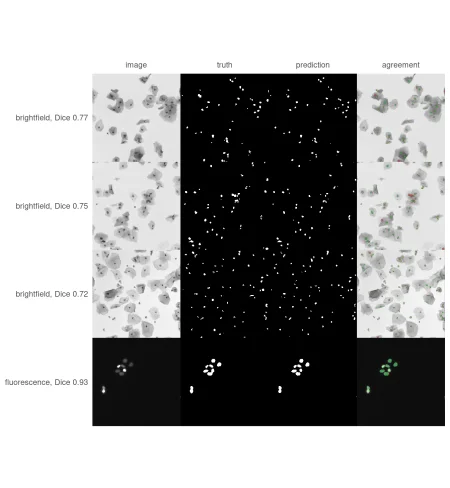
The low brightfield scores may reflect the imaging method, but the images suggest another possibility: nuclei may simply be too small after resizing. The brightfield images are 1024 by 1024 pixels, while the model processes each image at 256 by 256. A nucleus 16 pixels across in the original becomes about four pixels across on the model’s input grid. That leaves little detail for segmentation. To compare nucleus size on that same 256-pixel grid, measure the average mask area for each image type:nucleus_area <- function(case) {
files <- list.files(file.path(data_dir, case, "masks"), full.names = TRUE)
areas <- vapply(files, function(f) {
sum(read_masks(f, binary_colormap) == 2)
}, numeric(1))
size <- dim(read_masks(files[1], binary_colormap))[2:3]
mean(areas) * 256^2 / prod(size)
}
cases$area <- vapply(cases$case, nucleus_area, numeric(1))
aggregate(area ~ kind, cases, function(x) round(range(x)))
#> kind area.1 area.2
#> 1 brightfield 11 17
#> 2 fluorescence 69 957
#> 3 stained 137 1893
Resolution is the unresolved variable
The three weakest images share a problem the overall score can’t diagnose. Their nuclei average just 11–17 pixels on the measurement grid, while nuclei in the other image types start at 69 pixels. But those three images are also the only brightfield examples in the split, so there’s no way to tell whether the model struggles with brightfield images, tiny nuclei, or both.
The training set doesn’t break that tie: only 13 of its 536 images are brightfield, and all 13 are 1024 × 1024. The model’s predictions were made at 256 pixels, so scoring them at the original file resolution can’t restore the detail lost during resizing. Across 134 cases, the source resolution scores average 0.9208 Dice, with a 0.9314 median and a 0.7165 minimum. The worst case is 7f38885521586fc6011bef1314a9fb2aa1e4935bd581b2991e1d963395eab770. That mean is real; it just tells you little about the cases where the model falters.
The next useful comparison needs images where nuclei appear at their usual size. That means tiling instead of resizing, a subject for a later post in the series.
What the mean leaves out
Here’s the practical lesson: put the worst case beside the mean, then inspect what the weakest examples have in common. A single average hides the fact that this score is dominated by 105 fluorescence images and that the three worst images share two possible explanations. A per image table, plus a column you add yourself, made both visible with one function call and a few lines of R or Python.
If you report a segmentation score, report its weakest case too. The mean summarizes performance; the outliers tell you where to look next.
The series so far
- rplatypus rebuilt: deep learning for medical images in R covers why the 2020 package had to be rewritten, how it now installs its own Python, and how to create a first mask using the same published weights used here.
- Nuclei, five years later is this post.
Next, the series steps back from one dataset and looks at segmentation in rplatypus: four architectures, their differences, available losses and metrics, and the YAML file that describes an experiment field by field.
To leave a comment for the author, follow the link and comment on their blog: Data Science Guts.
R-bloggers.com offers daily e-mail updates about R news and tutorials about learning R and other topics. Click here if you're looking to post or find an R/data-science job.
Want to share your content on R-bloggers? Click here if you have a blog, or here if you don't.
Continue reading: Nuclei, five years later: what a mean Dice hides