Stratified Logistic Regression Keeps Imbalanced Data’s Predictions Interpretable

Why imbalance changes the picture

When one outcome is rare, logistic regression can produce fitted probabilities clustered near the majority class. That can make the model’s outputs harder to interpret, especially when those probabilities are used as propensity scores. A stratified modeling method offers a way to widen that range while retaining all observations: it repeatedly fits models with the minority class and a different portion of the majority class, then combines the estimates.

The approach is illustrated with U.S. student data from the OECD’s Programme for International Student Assessment. The dataset in R’s medley package contains 5,233 observations and 44 variables: 4,888 public school students and 345 private school students. Private school students make up about 6.6% of the sample.

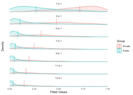
That imbalance matters for more than classification. In the example, increasing the ratio of public to private school students in a logistic regression narrows the distribution of fitted values toward the majority group. The accompanying figure shows the fitted-value distributions as the ratio rises from 1:1 to 14:1; each model includes all private school observations, while the number of public school observations increases.

One model per majority-class subset

Stratified modeling assigns each majority-class observation to one model and includes every minority-class observation in every model. The number of models depends on the class imbalance and the selected majority-to-minority ratio. With roughly 14 public school students for each private school student, a ratio of 1 produces 14 models. Public school observations appear once across the set; private school observations are reused.

The medley::stratified_glm() function fits these models. It accepts arguments for stats::glm(), but observation-specific arguments such as weights and subset can be unsuitable because each model receives a different subset of the data. The method is designed for binary classification, so the family defaults to a binomial model with a logit link.

results <- medley::stratified_glm(
  formula = Private ~ .,
  data = pisa,
  ratio = 1
)

To combine the model estimates, the method uses mitools::MIcombine, which applies Rubin’s Rules in this setting. The result gives a pooled coefficient and standard error. The individual model objects and fitted values are also available in the returned object, making it possible to inspect variation across models alongside the pooled summary.

For the PISA example, the reported coefficients with p-values below 0.1 include a positive estimate for the male indicator (0.84, standard error 0.28, p=0.004), and a negative estimate for ST08Q04TRUE (-0.50, standard error 0.27, p=0.071). Other displayed associations include ST08Q05TRUE (0.75, p=0.038), ST20Q06TRUE (1.79, p=0.060), and the response category “201-500 books” (1.18, p=0.050). These are model estimates from this example, not evidence that the method improves prediction by itself.

pisa_summary <- summary(results)
pisa_summary |> dplyr::filter(p < 0.1)

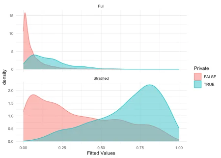
The fitted-value plot compares a conventional model using the full data with the stratified results. The stratified distribution spans more of the probability range, which the author argues makes the values easier to interpret. Predictions for new observations can be generated with predict(); the first six example predictions are 0.79, 0.16, 0.30, 0.24, 0.22, and 0.46.

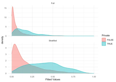
The choice of ratio affects the result. At a ratio of 3, the method is less effective at widening the fitted-value distribution than at a ratio of 1, as the accompanying plot indicates.

Prediction performance depends on the threshold

The article also tests whether the wider fitted-value range translates into better classification. It splits the data into 80% training and 20% validation sets, preserving the class balance: 93.4% public school students and 6.6% private school students in each partition.

On the validation set, the conventional logistic regression model has an area under the ROC curve (AUC) of 0.747. With equal costs assigned to false positives and false negatives, its accuracy-maximizing threshold is 0.465, yielding 93.4% accuracy. But that threshold gives a different picture from a threshold chosen where sensitivity and specificity intersect: at 0.059, accuracy is 66.4%, sensitivity 66.36%, and specificity 66.67%.

The stratified model’s AUC is 0.745, close to the full model’s result. Its threshold that maximizes accuracy is 1, with reported accuracy of 93.4%; at the sensitivity-specificity intersection of 0.509, reported accuracy is 68.6%. These figures underline the central distinction: changing the distribution of predicted probabilities doesn’t, by itself, improve the model’s ability to rank cases, as reflected in the similar AUCs. Classification results also depend heavily on the decision threshold.

There is a discrepancy in the article’s stratified confusion-matrix example: the code compares full_new_predictions with the stratified model’s intersection threshold, rather than comparing stratified_new_predictions with that threshold. The resulting matrix therefore should not be read as a clean evaluation of stratified predictions. As printed, it reports 93.22% accuracy, 99.69% sensitivity, and 1.45% specificity, a combination that also illustrates why accuracy alone can be misleading with a rare positive class.

Where the method may be useful

The practical case for stratification is strongest when the fitted probabilities themselves matter. Propensity score analysis, for example, uses logistic regression to estimate the conditional probability of receiving a treatment. If those scores are compressed toward the majority group, their range may be less useful for examining overlap between treatment and control groups. In the school example, private schools are the minority group and public schools the majority.

For ordinary classification, the evidence presented does not establish that stratified modeling is more accurate. A threshold tuned to the task can produce similar outcomes, and the reported AUCs are nearly the same. The method’s contribution is instead a different estimation structure that uses all majority-class observations across models and can yield a broader, more interpretable range of fitted values. Choosing the ratio and evaluating predictions with the correct model outputs remain essential to judging whether that tradeoff fits the analysis.