Bayesian Mixed-Effects Modeling for Repeated Biopsy Cell Composition Analysis

Repeated biopsies turn a simple cell proportion comparison into a problem of both composition and study design. Treat each phenotype as an independent outcome and average regions up to the patient, and you lose information about how cell types relate to one another and how measurements from the same person are connected. That matters in studies where each patient contributes several tissue samples over time.

sccomp is built for that setting. Its Bayesian mixed effects model works with cell counts, identifies outliers probabilistically, tests changes in variability, and accounts for unwanted effects. The input is a long tibble with one row per sample and cell type, plus counts and design columns. Its sccomp_estimate(), sccomp_test(), and sccomp_predict() functions return tibbles that fit into workflows using dplyr, tidyr, and ggplot2.

The NeoTRIP data

To show what this approach can do, Pierre-Paul Axisa, a researcher at CBMR in Copenhagen, applies sccomp to the NeoTRIP trial. Wang et al. (2023) used imaging mass cytometry to study how the spatial organization of triple-negative breast cancer relates to response to neoadjuvant immunotherapy. In phase III trial NCT02620280, patients with early high-risk TNBC were randomized 1:1 to eight three-week cycles of carboplatin plus nab-paclitaxel (C), either alone or with atezolizumab (C&I), followed by surgery. The source study is described in Wang et al. (2023).

The researchers collected formalin-fixed, paraffin-embedded biopsies at three stages: baseline (n = 243), the first day of cycle 2 (n = 207), and surgery after treatment (n = 210). A 43-marker panel measured tissue at subcellular resolution. Deep-learning segmentation and semi-supervised clustering identified 17 epithelial phenotypes and 20 tumor-microenvironment phenotypes, with multiple regions of interest (ROIs) imaged from each biopsy.

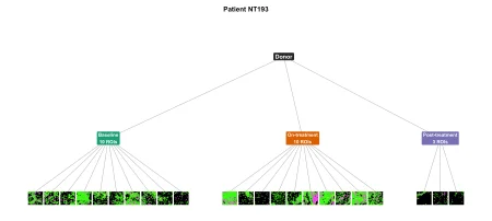
Here’s the key modeling issue: ROIs sit within biopsies, and biopsies sit within patients. Patient NT193, for example, was in the chemotherapy arm and had residual disease. The study imaged 10 ROIs at baseline, 10 during treatment, and three at surgery. Treating each ROI as a compositional sample while grouping repeated observations by patient preserves that structure in the analysis.

Wang and colleagues connected cell densities, spatial interactions, and proliferative fractions with pathological complete response (pCR). They also reported that immunotherapy changes tissue composition over time, with immune infiltration trajectories differing by response, including in their Figure 5. The dataset used here contains 257 per-protocol patients and 1,740 ROI-level immune samples. Each patient contributed a median of seven ROIs, and the analysis covers 15 immune cell phenotypes.

Why model the composition directly?

The original longitudinal analysis summarized phenotype proportions for each patient, then compared treatment arms, timepoints, and response groups using Wilcoxon tests, Z-scored trend plots, and phenotype-by-phenotype weighted binomial generalized linear models on tumor-level proportions. Those summaries make results easier to present, but they discard the ROI-level nesting and treat each phenotype separately. Since proportions must sum to one, a change in one cell type also changes the relative shares of others.

sccomp instead models ROI-level counts on a latent log-ratio scale, with mixed effects for both the mean and variability. Each ROI is the sample (sample = "ROI_id" in sccomp_estimate()); BiopsyPhase identifies the timepoint shared by multiple ROIs, and a patient intercept, (1 | PatientID), captures baseline differences between people while allowing estimates to shrink across the cohort. The data make the case for this structure more clearly than the method’s label does: the observations are repeated, nested, and compositionally constrained.

The analysis that follows uses tidyverse code to work from parsed input, focusing on the immune tumor-microenvironment compartment, ROI-level samples, and a patient random intercept. The long-format input has one row per ROI and immune phenotype, with ROI_id, a count, the design columns Arm, BiopsyPhase, and pCR, plus the grouping variable PatientID.

Reshaping the data for sccomp

The key step is turning the ROI measurements into a long table that keeps each cell count tied to its sample and clinical context. The analysis uses 1,740 regions of interest (ROIs) across 15 immune phenotypes. Each row records an ROI, a cell group and its count, alongside the patient ID, biopsy phase, treatment arm and response status. The R code reads `sccomp_long_tme_immune_roi.csv`, renames `sample` to `ROI_id`, converts counts to integers, and sets explicit category order: Baseline, On-treatment, then Post-treatment; C, then C&I; and RD, then pCR. That ordering makes the reference levels clear when the model is fitted. The preview shows, for example, ROI `NTImg0011` from patient `NT031`: it is a Baseline sample in the C&I arm from a patient with residual disease, with counts listed for immune groups including CD8⁺T and CD8⁺GZMB⁺T.

Fitting the model

The model asks how immune-cell composition varies across treatment arm, biopsy phase and response, including interactions among all three. Patient ID enters as a random intercept, accounting for the fact that a patient can contribute multiple samples. The variability formula is held constant, and `sccomp` uses a multi beta-binomial model with Hamiltonian Monte Carlo inference. It runs across the detected CPU cores. The output covers 1,740 samples and 15 cell groups, with 4,035 parameter rows. Its convergence summary reports effective sample sizes and split-chain R-hat values; the displayed rows show R-hat at 1.00. That’s a useful diagnostic, though the excerpt alone doesn’t establish how every parameter performed. The table also reports estimated composition effects, intervals, probabilities under the null, and false-discovery-rate adjusted values.

Comparing response groups after treatment

A proportional fold change gives a direct comparison of fitted proportions between two specified conditions. Here, the contrast holds treatment arm and biopsy phase fixed—C&I at post-treatment, or surgery—and compares residual disease with pathological complete response. The helper’s output is descriptive; statistical significance is evaluated separately by `sccomp_test()`. That distinction matters: a fold change summarizes the size and direction of a modeled difference, while the test supplies the inferential evidence.

Post-treatment differences are modest, with one clear exception

After treatment, the cell composition differs between patients with pathological complete response (pCR) and those with residual disease. The largest shift shown is in Tregs: their proportion is 3.4 times lower, falling from 0.0275 to 0.0081. CD56⁺ natural killer cells move in the opposite direction, rising 1.6-fold from 0.0808 to 0.1269. The other reported changes are smaller. CD4⁺PD1⁺T cells decline 1.6-fold, from 0.0439 to 0.0275; CD20⁺B cells fall 1.3-fold, from 0.0645 to 0.0496. CD4⁺TCF1⁺T cells decrease 1.1-fold, from 0.0918 to 0.0834, while CD79a⁺ plasma cells increase 1.1-fold, from 0.0721 to 0.0816. These estimates come with varying average uncertainty, and the table alone doesn’t establish whether the differences are statistically or clinically meaningful.

The model diagnostics look stable

The model’s 4,035 composition parameters show strong convergence: median is 1.001, with a maximum of 1.014. Their bulk effective sample size has a median of 4,837 and a minimum of 495; tail effective sample size has a median of 2,850 and a minimum of 923. Variability is modeled with one intercept per phenotype. Across those 15 coefficients, the maximum is 1.003, while minimum bulk and tail effective sample sizes are 3,404 and 2,451, respectively. Those diagnostics are reassuring overall. The composition parameters with the smallest bulk effective sample size are the next place to look when judging how much confidence to put in the estimates.