How to Build a Simplified MICE Imputation Workflow in R

MICE is easier to trust once you can see the machinery. This walkthrough builds a simplified version in R, step by step, and compares its results with the mice package. The author is candid that the code is experimental and the similarity may be luck; that’s part of what makes the exercise useful.

Why rebuild MICE?

Multiple imputation by chained equations is a familiar tool for handling missing data, but its inner workings can feel opaque. The author’s aim is to make the method less mysterious by implementing its basic steps from scratch in R—not by rebuilding ordinary least squares or maximum likelihood estimation, but by assembling the imputation process itself. Expect working code, rough edges, and more practical explanation than mathematical derivation. The Halloween references and pumpkins are the author’s; the central question is more serious: what does the software actually do when it fills in a gap?

What MICE does

A single replacement—say, filling every missing value with the mean—acts as though the guessed values were known. That can make standard errors too small. MICE instead creates several completed versions of the data, drawing plausible values for each gap so variation across the datasets reflects uncertainty in the missing information.

It does this through a sequence of conditional models. For each incomplete variable, the method predicts its missing values from the other columns, then passes those updated values along as it moves to the next variable. The cycle repeats; each completed dataset is analysed separately, and the estimates are combined using Rubin’s rules. The outline is straightforward. Getting the details right is where the work begins.

From simulated data to ten imputations

The example creates 1,000 observations in R. It generates three normally distributed predictors, two binary predictors, and a binary outcome whose probability depends on those predictors. It then introduces several kinds of missingness: random missing values in p1 and p3 (MCAR); missingness in p2 and p4 tied to other variables (MAR); and missingness in p5 tied to its own value (MNAR). The author links to a separate explanation of the missing data mechanism.

The hand-built procedure records which cells are missing, seeds them with random starting values, and processes each incomplete column in turn. For each column, it resamples observed rows, fits a linear regression for continuous data or logistic regression for binary data, then predicts the missing entries. Continuous predictions receive added residual noise; binary predictions become draws of zero or one from the estimated probabilities. Updated values feed into the next column’s model.

After ten passes through the columns, the code keeps the final values. It repeats this process across ten chains to produce ten completed datasets, fits the same logistic model to each—outcome ~ p1 + p2 + p3 + p4 + p5—and inspects the first fit with broom::tidy(). The author calls the result “pretty ok,” while acknowledging that parts of the code may be redundant. That modest claim fits the exercise: this is a learning implementation, and matching a package’s output doesn’t by itself prove every detail is correct.

The article’s roadmap continues from defining MICE and simulating data through the imputation procedure, pooling results, opportunities for improvement, and lessons learned. Its central value is the walk through the steps: if you work with missing data, seeing the chain operate can make the package’s “magic” easier to question and understand.

Pooling the models

The key test is whether a hand-built MICE workflow reproduces the package’s pooled results. It does: the author averages each coefficient across 10 fitted models, then combines within-model and between-model variance to calculate standard errors. Because the between-model variance comes from only 10 imputations, the 95% confidence intervals use Barnard–Rubin degrees of freedom and a t critical value. The R code below compares that calculation with `mice::pool()`, then plots both against a full-data fit, complete-case analysis, and the known coefficients used to generate the data.

library(mice)
imp <- mice(df_miss, m = 10, maxit = 10, seed = 1, printFlag = FALSE)
fit <- with(imp, glm(outcome ~ p1 + p2 + p3 + p4 + p5, family = binomial))
actual_mice_coef <- tidy(pool(fit), conf.int = TRUE) |>
select(term, estimate, std.error, conf.low, conf.high) |>
mutate(method = "actual_mice")

## function to grab stats
grab_stats <- function(df, method) {
model <- glm(outcome ~ p1 + p2 + p3 + p4 + p5, df, family = "binomial")
coef <- model |> tidy(conf.int = T) |> select(-statistic, -p.value) |> mutate(method = method)
return(coef)
}
## full data
full_data_coef <- grab_stats(df, "full_data")
## complete case
cco_coef <- grab_stats(df_miss, "complete_case")
## complete case analysis
all_coef <- rbind(mice_coef, full_data_coef, cco_coef, actual_mice_coef)
## truth
truth <- tibble(term = c("(Intercept)", "p1", "p2", "p3", "p4", "p5"),
truth = c(-0.5, 0.3, -0.2, 0.1, 0.5, 0.4))
## visualize all
all_coef |>
ggplot(aes(x = estimate, y = term, color = method)) +
geom_vline(xintercept = 0, linetype = "dotted", colour = "grey60") +
geom_pointrange(aes(xmin = conf.low, xmax = conf.high),
position = position_dodge(width = 0.6)) +
geom_point(data = truth, aes(x = truth, y = term),
inherit.aes = FALSE, shape = 4, size = 4) +
labs(x = "Estimate (log-odds)", y = NULL,
caption = "× = true coefficient") +
theme_bw()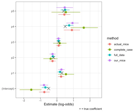

The comparison is reassuring: the from-scratch estimates track the `mice` package’s results across all coefficients, and both sit close to the fit using complete data. Their confidence intervals are a little wider, as they should be when missing values add uncertainty. Complete-case analysis discards rows with any missing value; here, its estimates drift farther and its intervals expand substantially. There are two details the chart can’t settle. Both MICE approaches put p4 somewhat above the full-data estimate, though their agreement points toward a feature of this sample rather than a pooling bug. And p5 was made missing not at random (MNAR), yet its estimates look reasonable. That apparent success may be chance in this one run; the result doesn’t establish that MICE handles MNAR data reliably. The author describes a long, uneven process of learning the method, including an early mistake: averaging the imputed datasets themselves instead of pooling the model estimates. The correction matters. Rubin’s rules combine estimates and their uncertainty across imputations; they don’t simply merge the completed data into one dataset.

What to improve next

The hand-built version is a useful way to understand the machinery, but there’s room to make it more faithful and easier to maintain. The author’s next steps are to sample from the posterior rather than resample, try predictive mean matching (the `mice` default, which uses observed values instead of adding normal noise), vectorize `missing_fill()`, keep state in lists rather than global variables, pass the random number generator explicitly, and run sensitivity analyses. The exercise also surfaced several pieces of R and statistical practice: `map2_dfc`, Rubin’s pooling rules, the total-variance formula, and Barnard–Rubin degrees of freedom. For anyone implementing imputation, the main lesson is practical: matching package output is a strong check on the pooling code, but it doesn’t make assumptions about the missingness mechanism disappear.

If you’d like to discuss the article or read more, visit the author’s blog. You can also follow them on BlueSky, Twitter, GitHub, or Mastodon, or get in touch about collaborating.

To comment, visit the original post: “r on Everyday Is A School Day”.

R-bloggers.com offers daily email updates with R news and tutorials, including learning R. It also links to R and data science jobs. Authors can submit a blog, or share content through r-posts.com.

Continue reading: My Messy Notes of Learning MICE From Scratch