R Guide to Converting Covariance and Correlation Matrices
Covariance and correlation describe the same pairwise relationships on different scales. In R, that makes converting between their matrices straightforward—but the direction of conversion determines what information you need. A covariance matrix contains both variable scales and their relationships; a correlation matrix keeps the relationships while removing the original units.
The distinction matters when comparing measurements with different units or moving between analyses that expect different matrix forms. In mixed models and time series analysis, for example, it can be useful to reconstruct one representation from the other. The mtcars dataset offers a compact example using miles per gallon, cylinders, displacement and horsepower.
What the two matrices show
Each row of mtcars represents a car, and its columns record vehicle characteristics. Here are the first six observations:
data(mtcars)
head(mtcars)
## mpg cyl disp hp drat wt qsec vs am gear carb
## Mazda RX4 21.0 6 160 110 3.90 2.620 16.46 0 1 4 4
## Mazda RX4 Wag 21.0 6 160 110 3.90 2.875 17.02 0 1 4 4
## Datsun 710 22.8 4 108 93 3.85 2.320 18.61 1 1 4 1
## Hornet 4 Drive 21.4 6 258 110 3.08 3.215 19.44 0 0 3 1
## Hornet Sportabout 18.7 8 360 175 3.15 3.440 17.02 0 0 3 2
## Valiant 18.1 6 225 105 2.76 3.460 20.22 1 0 3 1
For four of those columns, base R’s cov() function returns a variance-covariance matrix:
matr <- mtcars[,1:4]
Sigma <- cov(matr)
Sigma
## mpg cyl disp hp
## mpg 36.324103 -9.172379 -633.0972 -320.7321
## cyl -9.172379 3.189516 199.6603 101.9315
## disp -633.097208 199.660282 15360.7998 6721.1587
## hp -320.732056 101.931452 6721.1587 4700.8669
The diagonal entries are variances: each variable’s covariance with itself. The other entries describe how two variables vary together. A positive value means they tend to move in the same direction; a negative value means they tend to move in opposite directions. For instance, the covariance between mpg and disp is -633.0972.
Covariance values depend on the units and scale of both variables. That makes their magnitudes hard to compare directly across pairs. Pearson’s correlation standardizes covariance by dividing by the product of the variables’ standard deviations:
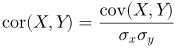
Correlation is bounded between -1 and 1, and each variable’s correlation with itself is 1. For these four columns, cor() gives:
R <- cor(matr)
R
## mpg cyl disp hp
## mpg 1.0000000 -0.8521620 -0.8475514 -0.7761684
## cyl -0.8521620 1.0000000 0.9020329 0.8324475
## disp -0.8475514 0.9020329 1.0000000 0.7909486
## hp -0.7761684 0.8324475 0.7909486 1.0000000
Convert covariance to correlation
For a single pair, the calculation uses only the covariance and the two variances on the diagonal. The covariance of mpg and disp, for example, becomes a correlation of approximately -0.8476:
-633.097208 / (sqrt(36.324103) * sqrt(15360.7998))
## [1] -0.8475514
Repeating that calculation for every pair would be tedious. The matrix form expresses the same operation compactly: divide each covariance by the standard deviation for its row variable and the standard deviation for its column variable. In matrix notation, place the reciprocal standard deviations on a diagonal matrix, then multiply the covariance matrix on both sides.
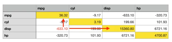
Pre-multiplying by a diagonal matrix scales rows. Post-multiplying scales columns. Since each covariance needs both adjustments, the steps are:
- Take the square roots of the diagonal variances to get standard deviations.
- Put their reciprocals on the diagonal of a matrix.
- Multiply the covariance matrix on the left and right by that matrix.
Here is the matrix calculation in R:
StDev <- sqrt(diag(Sigma))
StDevMat <- diag(StDev)
InvStDev <- solve(StDevMat)
InvStDev %*% Sigma %*% InvStDev
## [,1] [,2] [,3] [,4]
## [1,] 1.0000000 -0.8521620 -0.8475514 -0.7761684
## [2,] -0.8521620 1.0000000 0.9020329 0.8324475
## [3,] -0.8475514 0.9020329 1.0000000 0.7909486
## [4,] -0.7761684 0.8324475 0.7909486 1.0000000
That demonstrates the algebra, but base R already provides a direct function for this conversion: cov2cor().
cov2cor(Sigma)
## mpg cyl disp hp
## mpg 1.0000000 -0.8521620 -0.8475514 -0.7761684
## cyl -0.8521620 1.0000000 0.9020329 0.8324475
## disp -0.8475514 0.9020329 1.0000000 0.7909486
## hp -0.7761684 0.8324475 0.7909486 1.0000000
Two applications of sweep() provide another base R option, scaling once across rows and once across columns:
sweep(sweep(Sigma, 1, StDev, FUN = "/"), 2, StDev, FUN = "/")
## mpg cyl disp hp
## mpg 1.0000000 -0.8521620 -0.8475514 -0.7761684
## cyl -0.8521620 1.0000000 0.9020329 0.8324475
## disp -0.8475514 0.9020329 1.0000000 0.7909486
## hp -0.7761684 0.8324475 0.7909486 1.0000000
An outer product offers a concise element-wise expression. outer(StDev, StDev) forms a matrix containing every pairwise product of standard deviations, so dividing the covariance matrix by it produces correlations:

Sigma/outer(StDev, StDev)
## mpg cyl disp hp
## mpg 1.0000000 -0.8521620 -0.8475514 -0.7761684
## cyl -0.8521620 1.0000000 0.9020329 0.8324475
## disp -0.8475514 0.9020329 1.0000000 0.7909486
## hp -0.7761684 0.8324475 0.7909486 1.0000000
There is also a version using scale() and transposes. It applies the scaling in two passes, though its intent is less apparent when reading the code:
scale(t(scale(t(Sigma), center = F, scale = StDev)),
center = F, scale = StDev)
## mpg cyl disp hp
## mpg 1.0000000 -0.8521620 -0.8475514 -0.7761684
## cyl -0.8521620 1.0000000 0.9020329 0.8324475
## disp -0.8475514 0.9020329 1.0000000 0.7909486
## hp -0.7761684 0.8324475 0.7909486 1.0000000
Restore covariance from correlation
The reverse conversion follows directly from the same relationship: multiply each correlation by the standard deviations of its two variables. A correlation matrix alone doesn’t record those standard deviations, so they must be supplied separately. In this example, they come from the diagonal of Sigma.
For mpg and disp, multiplying -0.8475514 by the two standard deviations recovers a covariance of -633.0972:
-0.8475514 * sqrt(36.324103) * sqrt(15360.7998)
## [1] -633.0972
At the matrix level, place the standard deviations on a diagonal matrix and multiply the correlation matrix on both sides:
StDev <- sqrt(diag(Sigma))
StDevMat <- diag(StDev)
StDevMat %*% R %*% StDevMat
## [,1] [,2] [,3] [,4]
## [1,] 36.324103 -9.172379 -633.0972 -320.7321
## [2,] -9.172379 3.189516 199.6603 101.9315
## [3,] -633.097208 199.660282 15360.7998 6721.1587
## [4,] -320.732056 101.931452 6721.1587 4700.8669
For this task, the lavaan package provides cor2cov(), which accepts the correlation matrix and standard deviations:
lavaan::cor2cov(R, StDev)
## mpg cyl disp hp
## mpg 36.324103 -9.172379 -633.0972 -320.7321
## cyl -9.172379 3.189516 199.6603 101.9315
## disp -633.097208 199.660282 15360.7998 6721.1587
## hp -320.732056 101.931452 6721.1587 4700.8669
Alternatively, use sweep() to multiply the rows and columns by the standard deviations:
sweep(sweep(R, 1, StDev, FUN = "*"), 2, StDev, FUN = "*")
## mpg cyl disp hp
## mpg 36.324103 -9.172379 -633.0972 -320.7321
## cyl -9.172379 3.189516 199.6603 101.9315
## disp -633.097208 199.660282 15360.7998 6721.1587
## hp -320.732056 101.931452 6721.1587 4700.8669
The outer product makes the pairwise scaling explicit here too. Multiplying each correlation by the corresponding product of standard deviations reconstructs the original covariance matrix:
R * outer(StDev, StDev)
## mpg cyl disp hp
## mpg 36.324103 -9.172379 -633.0972 -320.7321
## cyl -9.172379 3.189516 199.6603 101.9315
## disp -633.097208 199.660282 15360.7998 6721.1587
## hp -320.732056 101.931452 6721.1587 4700.8669
A scale() and transpose formulation can perform the same operation, using reciprocal standard deviations as the scaling values:
scale(t(scale(t(R), center = F, scale = 1/StDev)),
center = F, scale = 1/StDev)
## mpg cyl disp hp
## mpg 36.324103 -9.172379 -633.0972 -320.7321
## cyl -9.172379 3.189516 199.6603 101.9315
## disp -633.097208 199.660282 15360.7998 6721.1587
## hp -320.732056 101.931452 6721.1587 4700.8669
The practical choice is simple: use cov2cor(Sigma) when converting a covariance matrix, and use lavaan::cor2cov(R, StDev) when the correlation matrix and standard deviations are available. The matrix identities explain why both conversions work; the standard deviations determine whether a correlation matrix can be returned to its original measurement scale.
Prof. Andrea Onofri
Department of Agricultural, Food and Environmental Sciences
University of Perugia (Italy)
Comments: andrea.onofri@unipg.it