Build an Orange Peel World Map with R’s Interrupted Goode Projection

Why use an interrupted Goode homolosine?

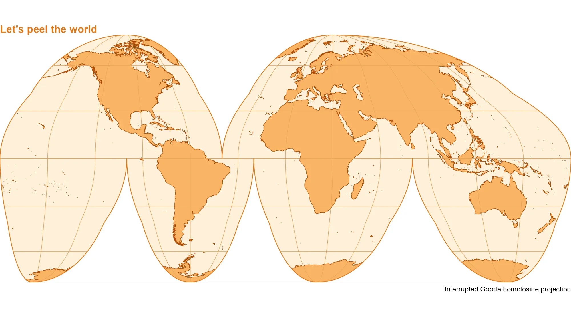
The interrupted Goode homolosine projection offers a useful visual tradeoff: it preserves relative area while splitting the map into lobes that reduce distortion across the world. That makes it a practical choice when comparing the sizes of regions matters, though the cuts interrupt the familiar continuity of a single rectangular world map. With a carefully drawn outline and graticules that stop at each cut, the result can resemble a flattened orange peel.

This shape is more than a visual flourish. A projection has to translate a curved surface onto a flat page, and that translation always changes some combination of area, shape, distance, or direction. Goode’s interrupted design spreads the distortions among separate regions rather than forcing the entire globe into one continuous outline. It’s a compromise with a clear purpose: keep areas comparable while making the map’s shape readable.

The interruptions do make construction more involved. Coastlines and grid lines need to follow the same boundaries, or the finished map can show stray lines bridging the gaps. Here’s the thing: the visual polish depends as much on managing those edges as on choosing the projection itself.

Prepare the outline and mask

This map uses three R packages: sf for spatial geometry and projection transforms, giscoR for coastal lines, and ggplot2 for rendering. Each package has a distinct job in the workflow: one supplies geometry operations, one retrieves the coastlines, and one assembles the layers into a figure. The first step retrieves the coastlines and defines the projection:

library(sf)
library(ggplot2)
library(giscoR)
world <- gisco_get_coastal_lines(resolution = 10)
goode_crs <- "+proj=igh"
lat <- c(90:-90, rep(c(-90:0, 0:-90), 3), -90:90, 90:0, 0:90, 90)
lon <- c(
rep(180, 181),
rep(c(80.01, 79.99, -19.99, -20.01, -99.99, -100.01), each = 91),
rep(-180, 181),
rep(c(-40.01, -39.99), each = 91),
180
)
outline <- st_sfc(st_polygon(list(cbind(lon, lat))), crs = 4326) |>
st_transform(goode_crs)
rectangle <- st_as_sfc(st_bbox(outline) * 1.1)
mask <- st_difference(rectangle, outline)

The coordinates for outline trace the edges of the interrupted shape in geographic coordinates, then st_transform() converts that geometry to the Goode projection. The small changes in longitude around the cut boundaries help define separate lobes instead of one uninterrupted perimeter. This is the structural part of the map: if the outline doesn’t describe the intended shape, later styling can’t repair the geometry.

Subtracting the outline from a slightly expanded bounding rectangle creates a mask that can cover anything outside the intended map shape, leaving the edges crisp. The rectangle is made a little larger than the outline’s bounding box so it extends beyond the artwork; the difference operation then leaves the area outside the outline available to cover underlying layers. That ordering matters because coastlines and grid lines may otherwise show beyond the shape. Small detail, visible result.

Keep the graticule inside each lobe

Drawing longitude and latitude lines across the full map would connect them through the projection’s cuts. Instead, the code defines six lobe boundaries, then builds meridians and parallels separately within each one. Small offsets at the edges help keep the lines from crossing the seams.

lobes <- list(
c(-180, -40, 0, 90), c(-40, 180, 0, 90),
c(-180, -100, -90, 0), c(-100, -20, -90, 0),
c(-20, 80, -90, 0), c(80, 180, -90, 0)
)
lines <- lapply(lobes, function(b) {
west <- b[1] + 0.01
east <- b[2] - 0.01
south <- max(b[3], -89.99)
north <- min(b[4], 89.99)
meridians <- seq(-180, 180, 30)
meridians <- meridians[meridians > west & meridians < east]
parallels <- seq(-60, 60, 30)
parallels <- parallels[parallels >= south & parallels <= north]
c(
lapply(meridians, function(x) {
st_linestring(cbind(x, seq(south, north, length.out = 181)))
}),
lapply(parallels, function(y) {
st_linestring(cbind(seq(west, east, length.out = 361), y))
})
)
})
grat <- st_sfc(do.call(c, lines), crs = 4326) |>
st_transform(goode_crs)

Each lobe is represented by its west and east longitude limits and its south and north latitude limits. The code uses those bounds to select which meridians and parallels belong in that region, then creates each line as its own geometry. This prevents the graticule from treating the cuts as if they were ordinary parts of the map.

The offsets of 0.01 degrees pull the line endpoints slightly away from the lobe edges, while the latitude limits avoid placing points exactly at the poles. The meridians and parallels are sampled at multiple points before projection, which gives the transformed curves enough intermediate coordinates to draw smoothly. Those choices are practical safeguards around a projection where edges and seams carry much of the visual structure.

If you’re working in this space, this is the part to inspect when seams look untidy: the grid is generated per lobe, so a boundary or sampling choice can affect one region without changing the rest. And this is the part most people overlook: a graticule is not merely decoration. It helps readers interpret geographic position, so its interruptions need to agree with the map’s underlying geometry.

Layer the map and finish the edges

The final plot combines a pale outline, orange filled coastlines, and a lighter graticule. The mask is drawn over the layers before the outline is traced, containing the artwork within the projection boundary. The order of the layers is doing real work here: the mask hides geometry outside the intended shape, and the final outline restores a clean edge on top.

ggplot() +
geom_sf(data = outline, fill = "#FFF0D9", colour = NA) +
geom_sf(data = world, fill = "#F9B566", colour = "#B34D08", linewidth = 0.25) +
geom_sf(data = grat, fill = NA, colour = "#E8A45B", linewidth = 0.25) +
geom_sf(data = mask, fill = "white", colour = NA) +
geom_sf(data = outline, fill = NA, colour = "#E87516", linewidth = 0.4) +
coord_sf(
crs = goode_crs,
xlim = st_bbox(outline)[c("xmin", "xmax")],
ylim = st_bbox(outline)[c("ymin", "ymax")],
expand = FALSE,
datum = NA
) +
theme_void() +
theme(
plot.background = element_rect(fill = "white", colour = NA),
plot.title = element_text(color = "#E87516", face = "bold")
) +
labs(
title = "Let's peel the world",
caption = "Interrupted Goode homolosine projection"
)

The coastlines use a stronger orange outline to separate land from the pale background, while the graticule uses a lighter shade so it remains visible without taking over the map. coord_sf() sets the projection and limits the displayed area to the outline’s bounding box. Setting expand = FALSE keeps extra padding from changing the framing, and datum = NA avoids adding a separate datum reference line.

The styling is deliberately restrained. This is more significant than it looks: a busy color scheme could make the interruptions harder to read, while a faint grid would leave viewers with little help judging location. The orange palette also supports the peel metaphor, though it doesn’t change what the projection preserves or distorts.

What the technique makes possible

This approach to outlining and masking follows Claus O. Wilke’s Interrupted Goode homolosine example. For a broader discussion of projections, Pyranhia’s French guide to cartographic projections offers another reference. Together, the examples point to a useful distinction: choosing a projection is one decision, while building a clean, readable map around it is another.

What this means for you is that the same workflow can be adapted when a map needs an unusual outline or carefully controlled internal lines. The general pattern is to define the boundary, construct the geographic features within its parts, transform them together, and use a mask to control what remains visible. Similar mapping tasks often benefit from treating seams as explicit geometry rather than relying on styling to hide them.

That said, the projection’s equal-area property comes with a tradeoff in shape and continuity, and the interruptions are part of that bargain. Readers should be able to see where the world has been divided and why the map looks unlike a familiar rectangular atlas view. A clear legend or accompanying explanation can help when the map is meant to support comparison rather than simply draw attention.

Useful, but not neutral.