R Function Selects the Largest Mainland Polygons from Map Data

For mapping workflows, a country boundary often includes islands and detached regions that get in the way of a mainland view. Those pieces may be geographically important, but they can dominate a map’s framing or distract from an analysis focused on the main landmass. A short R function built on terra can rank polygon or line features by size and return the largest ones, with optional controls for merging adjacent features and splitting multipart geometry.

The approach is deliberately simple: measure each feature, sort the measurements from largest to smallest, then keep the requested number. That makes it useful when a map needs a quick geographic filter and the largest feature is a reasonable stand-in for the area of interest. It’s a practical shortcut, though, not a test of whether a feature is truly a mainland.

Rank features by area or length

selectLargest() accepts a terra SpatVector containing polygons or lines. Set n to choose how many features to keep. With dissolve = TRUE, it aggregates the input before ranking; with singleparts = TRUE, it disaggregates multipart features. Polygons are ranked by area using terra::expanse(), while lines are ranked by length using terra::perim().

Those two options change what counts as a feature, so their order matters. Dissolving first can combine adjacent areas that would otherwise be ranked separately; disaggregating can then split multipart geometries into individual pieces. In the default settings, the function skips the dissolve and disaggregates multipart features, meaning a collection of disconnected pieces can compete as separate candidates.

Here’s the thing: the function ranks geometry, not political or geographic importance. A large island can outrank a smaller mainland, and a boundary dataset’s representation of adjacency can affect what gets merged. The result is only as useful as the assumptions behind the input and the chosen options.

selectLargest <- function(x, # terra SpatVector polygons or lines
                          n = 1, # number of largest features to retain
                          dissolve = FALSE, # whether to group contiguous features
                          singleparts = TRUE # whether to disaggregate multi-part features
                          ) {
  stopifnot(inherits(x, "SpatVector"),
            terra::geomtype(x) %in% c("polygons", "lines"))

  if (dissolve) {
    x <- terra::aggregate(x)
  }
  if (singleparts) {
    x <- terra::disagg(x)
  }

  if (terra::is.polygons(x)) {
    size_rank <- order(terra::expanse(x), decreasing = TRUE)
  } else if (terra::is.lines(x)) {
    size_rank <- order(terra::perim(x), decreasing = TRUE)
  }

  x[size_rank[1:n], ]
}

The input checks reject objects that aren’t SpatVector data and geometries that aren’t polygons or lines. That’s a useful boundary for a small helper function: it fails early when given an unsupported type instead of silently applying an unrelated measurement. The code then chooses the measurement based on geometry type and uses the resulting order to subset the original vector.

One detail deserves attention: n is used directly to select positions in the ranking. A caller should therefore choose a value that makes sense for the number of available features. This compact implementation doesn’t add separate handling for every edge case, such as an empty input or a request larger than the candidate set.

Examples across country maps

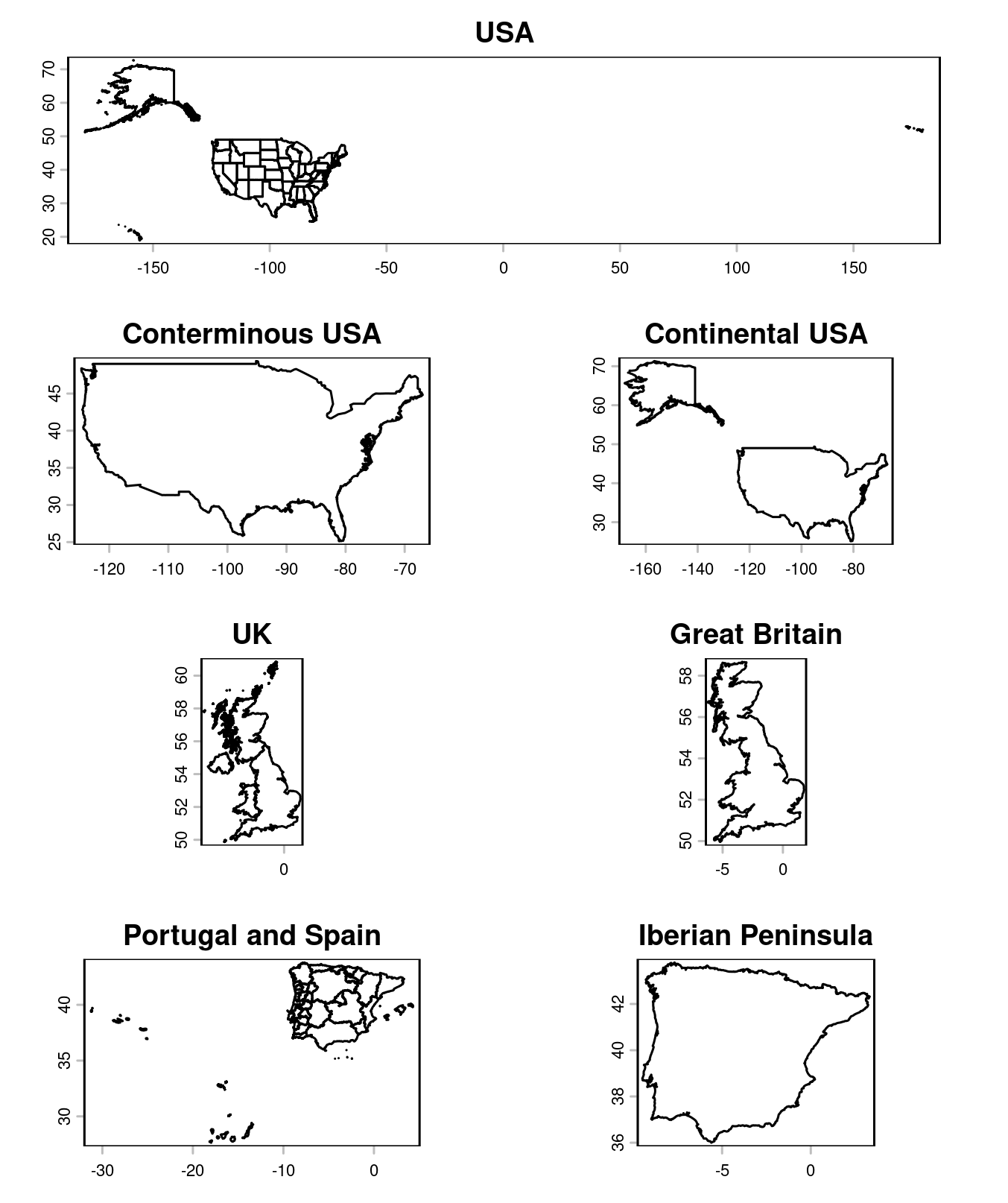
The examples use geodata::gadm() to load administrative boundaries. For the United States, selecting the largest dissolved polygon returns the conterminous area; requesting the two largest also includes Alaska. The same approach isolates Great Britain from the United Kingdom, or the Iberian Peninsula from a combined Portugal and Spain map.

The United States example shows why the choice of n is meaningful. Keeping one result selects the largest connected area after aggregation, while keeping two adds the next largest area. That can be a convenient way to make a mainland-focused map, but the function doesn’t know that Alaska is the intended second result; it simply ranks by measured area.

For the United Kingdom, the largest dissolved polygon corresponds to Great Britain in the example. Combining Portugal and Spain similarly produces a largest polygon associated with the Iberian Peninsula. These cases are clear demonstrations of the method because the desired map region aligns with the largest connected land area.

If you’re working with a different boundary dataset, inspect the geometries and their attributes before treating the output as a definitive geographic selection. Data sources can encode multipart boundaries and adjacent units differently. That said, the function gives you a concise, repeatable first pass, and the options let you adjust how it treats those structures.

library(terra)
library(geodata)

usa <- geodata::gadm("United States", level = 1, path = tempdir())
mainland_usa <- selectLargest(usa, dissolve = TRUE)
contin_usa <- selectLargest(usa, dissolve = TRUE, n = 2)

uk <- geodata::gadm("United Kingdom", path = tempdir())
great_britain <- selectLargest(uk, dissolve = TRUE)

ptes <- geodata::gadm(c("Portugal", "Spain"), path = tempdir())
iberia <- selectLargest(ptes, dissolve = TRUE)

The method makes “largest feature” a practical proxy for selecting a mainland, while leaving the number of retained features and treatment of borders configurable. This is more significant than it looks for routine map preparation: a small, explicit filter can make repeated workflows easier to understand and reproduce. Still, it’s a proxy. A single size ranking can’t replace a geographic decision when the target area isn’t simply the largest connected feature.

Where the shortcut helps—and where it stops

For quick visualization, the function can save manual selection and keep a map focused on its main area. It also gives analysts a consistent starting point when they need to process several boundary layers in the same way. The output remains a spatial vector, so it can be used in subsequent mapping steps without turning the selection into a purely visual edit.

And yet, area and length are blunt criteria. A larger feature isn’t automatically the one an analysis should retain, and changing whether the data are dissolved or split can change the ranking itself. For lines, the function ranks by perimeter length; that may fit some tasks, but the longest line feature isn’t necessarily the most relevant route or boundary.

(And this is the part most people overlook.) The function encodes a decision about what “largest” means before it encodes a decision about what “mainland” means. Check that the measurement and geometry handling match the map’s purpose, then review the selected features on the map. A useful filter, with assumptions attached.