Smoothing Reserving Issues: Harnessing Polars and Whittaker-Henderson for Chain-Ladder Analysis
A Reserving Problem, Solved Without Excel
When it comes to Chain-Ladder reserving, most actuaries associate the method with Excel or expensive software packages. An alternative approach, however, exists that leverages the modern capabilities of a dataframe library, enabling quick calculations for numerous insurers with minimal effort.
Using the CAS loss reserving data, focusing on the other liability line of business, we evaluated 233 US insurers. The data spans ten accident years, ranging from 1998 to 2007, encompassing paid and incurred losses throughout various development lags (1-10). For our analysis, we treated 2007 as the reporting year, simulating a year-end closure.
After ingesting the data, it undergoes necessary preparation:
import polars as pl
df = pl.read_csv("https://www.casact.org/sites/default/files/2026-03/othliab_pos_98-07.csv")
df_triangle = (
  df
  .group_by("GRNAME", "AccidentYear", "DevelopmentLag")
  .agg(pl.sum("IncurredLosses").alias("Incurred"), pl.sum("CumPaidLoss").alias("Paid"))
  .sort("GRNAME", "AccidentYear", "DevelopmentLag")
)
This format retains the "full triangle," capturing all ten development lags across the decade. It's formatted as a long data frame, in line with Tidy Data principles.
Implementing Chain-Ladder with Polars
The methodology follows traditional principles: aggregating claims by accident year and development lag, retaining only the upper-left triangle, and calculating Chain-Ladder development factors. These factors are derived through the formula:
f^{CL}_j = \frac{\sum_{i=1998}^{2008-j} C_{i,j}}{\sum_{i=1998}^{2008-j} C_{i,j-1}}In Polars, this process is streamlined using group_by and window expressions—eliminating the need for loops:
def df_2_cl_factors(df, group_by=None):
  g = [] if group_by is None else group_by
  cl_factors = (
    df
    .group_by(g + ["AccidentYear", "DevelopmentLag"])
    .agg(pl.sum("Paid"), pl.sum("Incurred"))
    .filter(REPORTING_YEAR >= pl.col("AccidentYear") + pl.col("DevelopmentLag") - 1)
    .sort(g + ["AccidentYear", "DevelopmentLag"])
    .with_columns(
      PreviousPaid=pl.col("Paid").shift(1).over(g + ["AccidentYear"]),
      PreviousIncurred=pl.col("Incurred").shift(1).over(g + ["AccidentYear"])
    )
    .group_by(g + ["DevelopmentLag"])
    .agg(
      number_of_years=pl.len(),
      Paid=pl.col("Paid").sum(),
      PreviousPaid=pl.col("PreviousPaid").sum(),
      Incurred=pl.col("Incurred").sum(),
      PreviousIncurred=pl.col("PreviousIncurred").sum()
    )
    .with_columns(
      f_CL_paid=pl.when(pl.col("PreviousPaid") == 0).then(1).otherwise(pl.col("Paid") / pl.col("PreviousPaid")),
      f_CL_inc=pl.when(pl.col("PreviousIncurred") == 0).then(1).otherwise(pl.col("Incurred") / pl.col("PreviousIncurred"))
    )
    .sort(g + ["DevelopmentLag"])
  )
  return cl_factors
cl_factors = df_2_cl_factors(df_triangle, group_by=["GRNAME"])
Validation against R’s ChainLadder package yielded consistent results for Grinnell Mutual Group, confirming our calculations.
Identifying Patterns That Don’t Fit
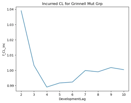
A closer inspection of individual company CL factors revealed anomalies. Two insurers raised red flags: Virginia Mutual Insurance Co showed an irregular paid development pattern, while Grinnell's incurred pattern failed to maintain monotonicity—an issue, as many commercial reserving tools assume monotonic behaviors which often suit parametric fits better. Grinnell's data journeyed above and below one, signaling shifts in reserves potentially impacted by case releases or subrogation.
Exploring Whittaker-Henderson Smoothing
Whittaker-Henderson (WH) smoothing serves as a non-parametric alternative, applying no fixed functional form, merely optimizing a balance between fit and smoothness. Its dual controls—penalty order and strength—allow fine-tuning based on the specific dataset.
This approach aligns perfectly with development factors, which can be interpreted as discrete-time signals with consistent intervals, a primary use case for WH smoothing that dates back over a century. As of scipy version 1.18, WH smoothing is readily available via scipy.signal.whittaker_henderson.
from scipy.signal import whittaker_henderson
f_smooth = whittaker_henderson(
  signal=f_cl_inc, weights=previous_incurred, lamb=1e4
).x
Notably, WH smoothing preserves the weighted in-sample sum, meaning smoothed factors yield precise replicas of observed incurred losses in the fitted section. However, discrepancies emerge in the un-sampled sections, which becomes significantly relevant for accurate reserving.
Impact on Reserve Estimates
The results indicated an approximate 3% adjustment in total reserves:
| accident year | reserve CL incurred | reserve smoothed |
| 1998 | 0.0 | 0.0 |
| 1999 | 7.5 | 20.6 |
| 2000 | 37.2 | 39.0 |
| 2001 | 21.5 | 38.3 |
| 2002 | 23.3 | 13.7 |
| 2003 | -124.9 | -118.9 |
| 2004 | -336.1 | -358.5 |
| 2005 | -522.0 | -525.9 |
| 2006 | -482.1 | -456.4 |
| 2007 | 394.4 | 398.2 |
| -981.1 | -950.0 |
This suggests a modest shift in total reserves, with some individual accident years adjusting significantly due to the smoothing effect enabling neighboring factors to influence values.
In comparison to the incurred losses after the full term development, both unmodified and smoothed Chain-Ladder methods exhibit slight overestimations. Yet, the unmodified approach proved marginally closer to actual figures.
| incurred | ultimate CL | ultimate smoothed |
| 189,901 | 194,067 | 194,098 |
While smoothing enhances interpretability of data, it may not necessarily yield greater forecast precision—underscoring the vital need for comparative validations.
Key Takeaways
- Polars offers an efficient framework for Chain-Ladder computations, facilitating swift analysis across numerous insurers simultaneously.
- Volume-weighted CL factors derived in Polars align perfectly with results from R’s
ChainLadderpackage, instilling confidence during tool transitions. - Whittaker-Henderson smoothing presents itself as a valuable alternative to parametric curve fitting, especially for handling noisy or non-monotonic development factors. Nevertheless, accuracy must always be cross-checked with holdout data when practicable.
Future enhancements could involve integrating a tail factor, assessing reserve uncertainties (like Mack's method), or automating lamb selection using REML techniques.
The complete notebook, featuring all requisite Polars code, visualizations, and comparisons to R results, is available on GitHub. This post, along with the notebook, has undergone AI review.
If you notice any issues or possess preferred methods for smoothing development factors, your thoughts in the comments would be appreciated!