Cleaning 49,000 Personality Survey Responses in R: Age Filters and Careless-Response Flags

Most psychometric write-ups skip straight to the reliability coefficients and factor loadings. That's a shame, because the data prep is where the analysis is won or lost. A scale can look clean after the model runs, but if a few thousand straight-liners and impossible ages are sitting in the file, the results mean much less than they appear to. This walkthrough covers how I'd clean a large, uncontrolled personality dataset before running any classical or Rasch analysis.

The dataset and its quirks

The data comes from the Open-Source Psychometrics Project, which hosts a range of personality measures and makes the responses freely available. This particular file covers Cattell's 16 Factor Personality Measure, using items from the International Personality Item Pool (IPIP) chosen to reflect Cattell's 16 factors. The file loads as 49,159 rows and 169 columns: 168 numeric item responses plus a country variable.

The codebook that ships with the download is a data dictionary. It tells you each variable's name, definition, and coding, but it doesn't flag which items are reverse-keyed. That information lives on a separate IPIP key page, which lists the items for each scale in order, marks the reverse-keyed ones, and reports the alpha for each scale from the original research. Grab that page before you touch the data. You'll need it when you start scoring, and it gives you a benchmark for checking your own reliability estimates later.

Here's the thing about data like this: the cleaning decisions depend on how it was collected. A testing-center sample and an open online survey carry very different risks. This was an online survey, and none of the items were required. That means missing data is expected, straight-lining is likely, and age is a free-text field that anyone can fill with nonsense.

library(tidyverse)
library(ggthemes)
PF16 <- read_tsv("data.csv")

The age problem

The website documentation says anyone under 13 was removed from the downloadable set, along with anyone who opted out of data sharing. That leaves 13- to 17-year-olds in the file, which is fine on its own terms. The real trouble is the respondent who entered 2,147,483,647 as their age. That number is roughly two billion years, which would place their birth somewhere in the Paleoproterozoic era, back when the only living things on Earth didn't need oxygen. It's a funny answer. It's also a warning sign, because someone who types nonsense into the age box has probably typed nonsense into the 168 items too.

Before deciding on a cutoff, I'd look at the distribution of the highest ages:

PF16 %>%
  filter(age > 99) %>%
  group_by(age) %>%
  summarise(count = n())

A quick check against published records helps set the threshold. The oldest verified person on record lived to 122, and the oldest living person is 117. Respondents claiming to be older than that are almost certainly not reporting accurately. I'd set the line at 102, which sits comfortably above what's biologically plausible for a living respondent and still leaves room for a few people who were just rounding up. The cutoff is a judgment call, but it's an explainable one.

There's a limit to this logic, though. Plenty of people probably shaved years off their age or lied outright for reasons that have nothing to do with the measure. Without direct evidence that a specific respondent was lying, I'd leave them in. Filtering on a plausible age ceiling removes obvious garbage. Trying to guess who's fibbing about being 35 versus 38 just adds noise of your own.

PF16 <- PF16 %>%
  filter(age <= 102) %>%
  mutate(ID = row_number(),
         age_group = cut(age,
                         breaks = c(12, 17, 24, 34, 44, 64, Inf),
                         labels = c("13 to 17", "18 to 24", "25 to 34",
                                    "35 to 44", "45 to 64", "65+"),
                         right = TRUE))

The cut() call deserves a note because it trips people up. With right = TRUE, each break value is the upper end of its interval, so the first break has to be one below the minimum age you want to include. That's why the vector starts at 12 to capture 13-year-olds. Get this wrong and your age groups will be off by one with no error message to warn you. I always check the group counts after cutting.

Also, I'm assigning row numbers as IDs. Each row is one respondent, so that's a clean identifier for joining the flag data back later.

Recoding missing responses

In this file, skipped items were coded as 0. R will happily treat 0 as a valid response, which would quietly bias any mean or correlation. Converting those to NA across the item columns fixes it in one line:

PF16 <- PF16 %>%
  mutate(across(A1:P10, ~na_if(., 0)))

The across() call works here because the items sit side by side in the file, so a single range covers them all.

Finding careless responders without punishing honest ones

This is where judgment matters more than any package. Careless responding includes straight-lining (picking the same option every time) and alternating between two options, like 4-5-4-5 down the page. Those patterns tell you nothing about the trait being measured. But a volunteer online survey is a messy context. Someone might be bored, or they might be confused by a poorly worded item. Someone else might be a student who was required to finish the measure for a class and just wanted it over with. Those are different situations, and the data can't tell you which one you're looking at.

Given that uncertainty, I'd rather be conservative. Dropping a truly careless respondent costs you very little. Dropping a respondent whose "careless" answers were really a reaction to a bad item can distort your validation work. So the goal is to catch the clearest cases and leave the ambiguous ones alone.

Two indices from the careless package do most of the work here. The longstring index counts the longest run of identical answers in each row. The intra-individual response variability (IRV) measures how much each row's responses vary, and it's better at catching people who bounce between two adjacent options. The package is easy to install with install.packages("careless") if you don't already have it.

I like to build a separate tibble of item responses only, so none of the demographics or IDs leak into the calculations:

library(careless)

Items <- PF16 %>%
  select(A1:P10)

longstrings <- longstring(Items, avg = TRUE)

Flags <- tibble(
  ID = PF16$ID,
  longstring = longstrings$longstr,
  avgstring = longstrings$avgstr,
  irv = irv(Items, na.rm = TRUE),
  na_count = rowSums(is.na(Items)),
  pct_long = longstring / 163
)

The pct_long column divides the longest string by 163, the total number of items. That gives you the share of a respondent's answers that fell inside one unbroken run. The 163 comes from the scale structure: fifteen scales with 10 items each, plus scale B (intellect) with 13.

Setting the thresholds

I'd start with IRV, since it's the best single signal for the most extreme cases. A histogram makes the distribution easy to read:

Flags %>%
  ggplot(aes(irv)) +
  geom_histogram() +
  theme_economist_white()

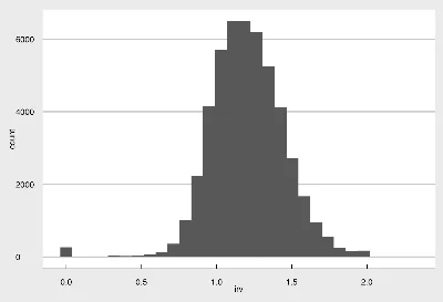
There's a clear spike of cases at an IRV of 0. Those are the true straight-liners, and there's no reasonable argument for keeping them. A bit further along, there's a smaller cluster at 0.50 or below, which corresponds to people who alternated between two options. The counts are low, so a cutoff at 0.50 costs you very little. Applying it dropped 381 cases:

Flags <- Flags %>%
  filter(irv > 0.50)

The longstring percentage is harder to call. The observed values run from about 0.6% to just under 44%, and the distribution has a long right tail. I plotted it with a bin width of 1 percentage point, capped the x-axis at 50%, and looked for a natural break:

Flags %>%
  ggplot(aes(pct_long)) +
  geom_histogram(binwidth = .01) +
  scale_x_continuous(limits = c(0, 0.50)) +
  theme_economist_white()

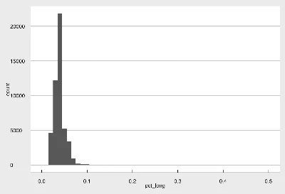
The counts drop sharply around 9%. A 9% cutoff corresponds to a longest string of 15 responses, and 10% corresponds to 17. I checked both by filtering and printing the results. At 9%, 335 cases would be flagged. At 10%, that drops to 265.

Here's where I'd push back on my own instinct. The scales have 3 to 5 reverse-keyed items each. If those items are working as designed, a careful respondent's longest run of identical answers shouldn't exceed about 8. So a string of 15 or more is already suspicious. But that reasoning assumes the reverse-keyed items are functioning as intended. If a negatively worded item is actually unrelated to the trait, a string of 15 could reflect a bad item rather than a bad respondent. That's exactly the scenario the conservative approach is designed to protect against.

The sample also makes the decision easier. Going with 10% removes only about 0.5% of the total sample. Given that, I'd take the more conservative cutoff and keep the marginal cases:

Flags <- Flags %>%
  filter(pct_long < 0.1)

Handling missing data

The last filter deals with missingness. Here's the distribution of missing items per respondent:

NAs <- Flags %>%
  group_by(na_count) %>%
  summarise(count = n())

head(NAs)

Keeping only complete cases would still leave more than 35,000 respondents, which sounds like plenty. But the psychometric methods I'm planning to use, classical test theory and Rasch modeling, can handle a modest amount of missing data. Throwing away every respondent with a single skipped item would discard a lot of usable information for no good reason. I'd set the cutoff at two or fewer missing responses. That keeps most of the sample, and it shouldn't meaningfully affect the validation of these scales.

Flags <- Flags %>%
  filter(na_count <= 2)

Now I can apply all the flag-based decisions to the main dataset in one step:

PF16 <- PF16 %>%
  filter(ID %in% Flags$ID)

write_csv(PF16, "Cleaned PF16 Data.csv")

What this gets you

The cleaned file is smaller, but it's a more defensible starting point. Every exclusion has a stated rule behind it: an age ceiling tied to documented human lifespans, an IRV floor for straight-liners and two-option alternators, a longstring cutoff set where the distribution breaks, and a missingness limit that keeps the sample usable. None of those rules is perfect, and each one involves a tradeoff between removing noise and removing real respondents.

The bigger lesson is that the flagging thresholds should be documented and, ideally, tested. Rerunning your analysis with the 9% cutoff alongside the 10% one would show whether your reliability estimates are sensitive to the choice. If they barely move, you can stop worrying. If they shift, you've learned something important about how much those careless-looking patterns are shaping your results.

Next up is the classical test theory analysis, which is where the cleaned data starts to show whether these 16 scales hold together. My expectation is that the cleaning choices will matter less than the reverse-keyed items, and that's the part I'll be watching most closely.