Build Reliable AI Agents in R by Delegating Data Counts to Code

Why the counting needs to leave the model

A model can sound certain and still give you numbers you can’t verify. Asked twice how many people in a clinical trial’s high dose group had itching, Gemini answered 21 and then 25. It cited trial data files, but it hadn’t been given those files. The mismatch points to a practical limit of chatbots: confident prose doesn’t tell you what data—or what definition—the answer came from. This is the opening installment of a five part series about putting AI agents into production with R. The example is a clinical trial safety assistant, and each installment builds on the same app: - [From Chatbot to Agent](https://www.jumpingrivers.com/blog/agents-in-production-first-agent/) (this post) - Putting the Agent in a Shiny App - Can You Trust It? - Audit Trails, Costs and Models - Sharing Your Tools with MCP The series’ answer to unreliable arithmetic is simple: let the model choose an R function, then let R do the counting. The model is told not to calculate for itself, and a later installment checks whether it follows that rule. That still leaves room for the model to ask the wrong question, so the assistant reports the filters behind every result. If you work with data, that distinction matters: a count is only useful when you know what was counted. No pharmaceutical background is needed. The same pattern can apply wherever a team asks questions about data. Later parts add a Shiny app, tests, controls over who can see patient records, an audit trail, and a way to share tools with other AI agents. ## What makes an AI agent different? A chatbot produces answers from patterns learned during training. An agent can also request that your code perform a task, a capability called tool or function calling. You give the model tools with names, descriptions, and arguments. If it needs one, it sends a request such as `count_subjects()` with `arm = "Placebo"`. Your R session runs the function and returns its result. The model can request another tool, then use the returned information to answer. That back and forth is the agent loop. The boundary is important: **the model doesn’t execute your code.** It asks; your R session decides what runs and what information comes back.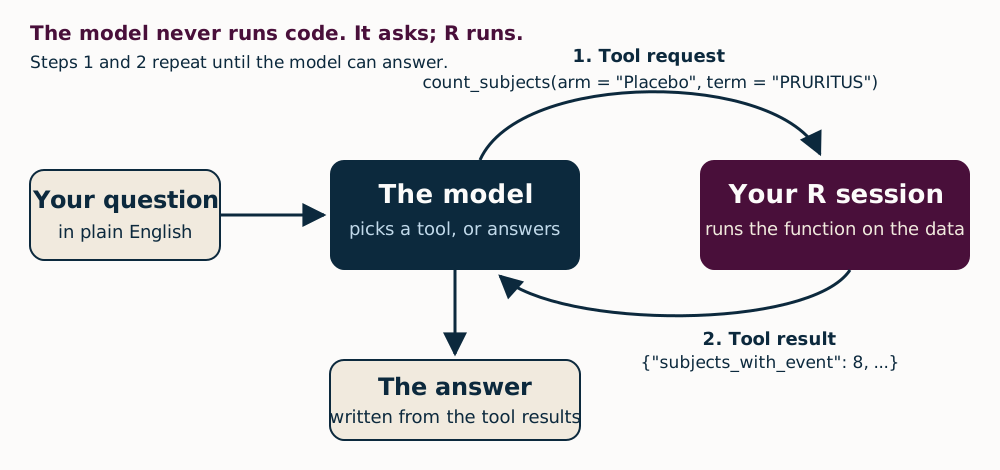

The R package {ellmer} handles this loop. You write regular R functions, describe them, and register them with a chat. If {ellmer} is new to you, the [LLMs in R & Python webinar](https://www.jumpingrivers.com/blog/programming-llms-r-python/) is a place to start. The [{ellmer} tool-calling guide](https://ellmer.tidyverse.org/articles/tool-calling.html) recommends keeping exact computation inside the tools. ## Setup and access The code for this installment is in [the blog repository](https://github.com/jumpingrivers/blog/tree/main/blogs/agents-in-production/part-1). Clone the repository or download it as a ZIP, then open the project in R 4.5. To restore the package versions pinned by {renv}, run:

install.packages("renv")
renv::restore()

You can install the packages yourself instead, though those versions may be newer than the ones tested:

install.packages(c("ellmer", "pharmaverseadam", "dplyr", "jsonlite"))

You’ll also need a Gemini API key. The [alt-text post](https://www.jumpingrivers.com/blog/ellmer-dynamic-alt-text/) explains how to get one. Store the key by running `file.edit(".Renviron")` in the project, adding `GEMINI_API_KEY=your-key`, saving the file, and restarting R. The code README includes further setup notes, particularly for Windows. The free tier works for this example because the trial data is public. That doesn’t make it suitable for patient or confidential information. Google’s terms also require a paid service for apps offered to users in the UK, EEA, or Switzerland; the series returns to this in part four. The authors tested with R 4.5.1, {ellmer} 0.5.0, and {pharmaverseadam} 1.3.0 in September 2026. Since {ellmer} changes quickly, version differences are one thing to check if the code behaves differently. ## The trial behind the example The assistant uses CDISC pilot study 01, a worked example published by CDISC, the organization that sets clinical trial data standards. The study tested a skin patch containing experimental drug xanomeline in people with mild to moderate Alzheimer’s disease. Participants, called *subjects* in the trial data, received placebo, a low dose, or a high dose for 26 weeks. The {pharmaverseadam} package rebuilds the study’s analysis datasets in CDISC’s ADaM format. This example uses `adsl`, one row per subject, and `adae`, one row per adverse event. An adverse event is an unwanted medical occurrence during the trial; it doesn’t have to be caused by the drug. A few definitions shape the counts: - **Arm:** a treatment group: placebo, low dose (54 mg), or high dose (81 mg, after two weeks at 54 mg). - **Screen failure:** someone assessed for the trial who did not join. - **Safety population:** everyone who received at least one dose; safety results use this group. - **Treatment-emergent event:** an event that began or worsened after the first dose and within a defined period after the last dose. Here that period is 14 days. - **Serious adverse event:** an event with an outcome such as death, a life threat, hospitalization, or lasting disability. Severity is recorded separately as mild, moderate, or severe; a severe headache need not be serious. The `AESER` flag marks serious events, and the tools count that flag. - **Preferred term and body system:** MedDRA codes each event using standard medical terminology. “Itchy skin” becomes the preferred term PRURITUS, under “skin and subcutaneous tissue disorders.” - **Application site:** the place where the patch was worn. Erythema means redness. 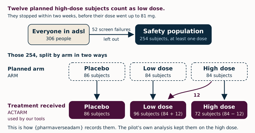Here’s the thing: the population and treatment assignment can change the answer as much as the event definition does. The `adsl` dataset has 306 people, including 52 screen failures, leaving 254 in the safety population (`SAFFL == "Y"`). Each subject has a planned treatment (`ARM`) and a received treatment (`ACTARM`). Twelve people assigned to high dose stopped before the dose increased to 81 mg, so this example counts them with the low dose.

The treatment-emergent filter (`TRTEMFL == "Y"`) reduces 1,191 adverse-event rows to 1,122. The project’s `R/data.R` function applies these filters and selects the subject and event fields the tools need:

ARMS <- c("Placebo", "Xanomeline Low Dose", "Xanomeline High Dose")
load_trial_data <- function() {
subjects <- pharmaverseadam::adsl |>
dplyr::filter(SAFFL == "Y") |>
dplyr::select(USUBJID, ACTARM, AGE, SEX, RACE)
events <- pharmaverseadam::adae |>
dplyr::filter(TRTEMFL %in% "Y", USUBJID %in% subjects$USUBJID) |>
dplyr::select(USUBJID, ACTARM, AEDECOD, AETERM, AEBODSYS, AESER, AESEV, ASTDT)
list(
subjects = subjects,
events = events,
# Every term and body system recorded in the trial, including the few
# never treatment-emergent, so asking about them gives a real zero.
terms = sort(unique(pharmaverseadam::adae$AEDECOD)),
body_systems = sort(unique(pharmaverseadam::adae$AEBODSYS))
)
}

For readers who work in pharma, the [note for pharma readers](https://www.jumpingrivers.com/blog/agents-in-production-first-agent/#a-note-for-pharma-readers) discusses choices a formal analysis plan might handle differently. ## What a model guesses without tools The authors asked `gemini-3.7-flash` the same question twice without registering any tools:

# Without tools, the model can only guess.
bare <- ellmer::chat_google_gemini()
bare$chat("In CDISC pilot study 01, how many subjects on high-dose xanomeline had pruritus?", echo = "output")

Pruritus means itching. The answers below are reproduced as returned, including their Markdown, with headings shown in bold. Neither response matches the project’s calculation. The figures are revealing because each contains a number that looks plausible for a different reason: | Result | High-dose pruritus | What it represents | |---|---:|---| | First answer | 21 of 84 (25.0%) | The low-dose count divided by the planned high-dose group size | | Second answer | 25 of 84 (29.8%) | The right count divided by the planned group size | | Project data | 25 of 72 (34.7%) | Treatment-emergent cases, grouped by treatment received | For placebo, the data gives 8 of 86 (9.3%); the other figures in the two model answers don’t match the data either. The second answer is particularly easy to accept: its count is correct, while its denominator is wrong. Neither response identifies the population, data, or event rules behind its figures. A quick plausibility check could miss the problem. ## Building the counting tool The model sees a tool’s description, not its R implementation, so that description helps determine when it gets called. Most of the counting happens in `count_subjects()` in `R/tools.R`:

count_subjects <- function(data, arm = NULL, serious_only = FALSE, term = NULL, body_system = NULL) {
arm <- check_arm(arm)
serious_only <- check_flag(serious_only, "serious_only")
term <- check_known(
check_string(term, "term"), data$terms, "preferred term",
"Call ae_summary to see the terms used in this trial."
)
body_system <- check_known(
check_string(body_system, "body_system"), data$body_systems, "body system",
"Call ae_summary with by = 'body_system' to see them."
)
data <- filter_arm(data, arm)
events <- data$events
if (serious_only) events <- dplyr::filter(events, AESER == "Y")
if (!is.null(term)) events <- dplyr::filter(events, AEDECOD == term)
if (!is.null(body_system)) events <- dplyr::filter(events, AEBODSYS == body_system)
n <- dplyr::n_distinct(events$USUBJID)
total <- nrow(data$subjects)
jsonlite::toJSON(list(
arm = arm %||% "All arms",
# Say what was counted, so a wrong reading of the question shows.
filters = list(
serious_only = serious_only,
term = term %||% "any",
body_system = body_system %||% "any"
),
subjects_with_event = n,
subjects_in_arm = total,
percent = round(100 * n / total, 1)
), auto_unbox = TRUE)
}

Four implementation choices carry much of the safety burden: - **JSON output:** the model reads text, and {ellmer} 0.5.0 deprecates returning data frames from tools. - **Visible filters:** each result reports the filters applied, so a misread question can be spotted. - **Unknown values fail:** requesting a term that isn’t in the trial raises an error with instructions for recovery. Treating “I didn’t understand” as a count of zero would be worse. - **Arguments are checked:** models can send values in unexpected types. The checks also matter when other programs call these tools through MCP, the standard for sharing tools between AI applications, in part five. That last guard came from testing: passing `serious_only = "true"` as text instead of `TRUE` silently counted every subject with any adverse event, returning 217 rather than 3. Because the function is ordinary R, you can also call it without an AI model. Source the files in `R/` first:

for (file in list.files("R", pattern = "[.]R$", full.names = TRUE)) source(file)
count_subjects(load_trial_data(), arm = "Xanomeline High Dose", term = "PRURITUS")
#> {"arm":"Xanomeline High Dose","filters":{"serious_only":false,"term":"PRURITUS","body_system":"any"},"subjects_with_event":25,"subjects_in_arm":72,"percent":34.7}

The tool registration tells the model what it can request:

ellmer::tool(
function(arm = NULL, serious_only = FALSE, term = NULL, body_system = NULL) {
count_subjects(data, arm, serious_only, term, body_system)
},
name = "count_subjects",
description = paste(
"Count subjects in the safety population with at least one treatment-emergent",
"adverse event matching the filters. Returns the count, the number of subjects",
"in the arm and the percentage."
),
arguments = list(
arm = arm_type,
serious_only = ellmer::type_boolean("Only count serious adverse events.", required = FALSE),
term = ellmer::type_string(
"MedDRA preferred term, e.g. 'PRURITUS'. Leave out to count any event.",
required = FALSE
),
body_system = ellmer::type_string(
"MedDRA body system, e.g. 'NERVOUS SYSTEM DISORDERS'. Leave out for any.",
required = FALSE
)
),
annotations = ellmer::tool_annotations(title = "Counting subjects", read_only_hint = TRUE)
)

The arm argument is an enum, meaning the model is shown the three allowed values:

arm_type <- ellmer::type_enum(ARMS, "Treatment arm. Leave out to cover all arms.", required = FALSE)

`check_arm()` also rejects invalid values if a caller ignores that list. The project’s `trial_tools()` function creates four tools around one copy of the data: `list_arms()` for group sizes, `ae_summary()` for common events, `count_subjects()` for filtered counts, and `subject_profile()` for an individual patient’s record. ## Starting the agent loop A short function in `R/agent.R` assembles the agent: it creates a Gemini chat with the system prompt, introduced in the next section, and registers the tools.

What the tools change

The key result here is that the agent’s answers can be traced back to actual counts. Asked to compare adverse events for 72 people on high dose with 86 on placebo, it requested the ten most common events in each arm. Four events in the high dose list weren’t in the placebo list, so it checked those individually with `count_subjects()`. Pruritus topped the high dose results: 25 people (34.7%), versus 8 (9.3%) on placebo. Application site pruritus affected 21 (29.2%) versus 6 (7.0%); application site erythema, 14 (19.4%) versus 3 (3.5%). The full high dose list also included erythema, dizziness, application site irritation, hyperhidrosis, rash, sinus bradycardia and application site dermatitis, with placebo comparisons shown in the agent’s answer above. That pattern makes the skin reactions hard to miss, though the counts alone don’t explain their cause. For serious adverse events, the tool counted three people across all 254 participants: two of 96 in the low dose arm, one of 72 in the high dose arm, and none of 86 on placebo. Those figures describe the dataset’s `AESER` flag; they don’t tell the whole story of events that might meet other seriousness criteria. Here’s the practical point: the model chose the queries, but R returned the counts. Every number in these answers appears in a tool result. That’s a much stronger basis for trust than a prompt asking the model to be careful, though the later parts of the series add checks because prompts can still be ignored.

Where the agent still needs guardrails

The system prompt tells the model to use tools for every trial fact, quote their numbers exactly, identify the arm and population, and admit when the tools can’t answer. Those rules set a useful standard. They don’t enforce it. Part 3 adds a check that verifies where each answer’s numbers came from. The choice of tools matters too. A single `run_r_code()` function would let the model write arbitrary analysis code, leaving the team to validate whatever it produced. Smaller functions such as `ae_summary()` and `count_subjects()` are easier to test against hand-checked results, log and control. They also reduce the model’s job to selecting a query instead of composing correct `{dplyr}` code. Several operational issues remain. The model can currently open any patient record; part 3 restricts `subject_profile()` to a reviewer group, and part 5 excludes it from tools shared with other AI agents. A console session serves one person, while part 2 gives each Shiny user a separate conversation. Provider limits are another constraint: the free tier returned “503 high demand” and “429 quota exceeded” errors within minutes. At the time of writing, it allowed about 20 requests per model per day. A question can take one request for each round of tool calls, and `{ellmer}` retries each request up to three times by default; `options(ellmer_max_tries = …)` changes that. Parts 2 and 4 address the remaining issues. The model setup is flexible, but its default can move. With `model = NULL`, `{ellmer}` 0.5.0 selects `gemini-3.7-flash`; part 4 pins a model by name. Switching providers usually means changing one argument, as in `make_agent(chat_fun = ellmer::chat_anthropic)`. Local models via `chat_ollama()` have an additional catch covered in that later part. You can run the demo with `source("demo/part-1.R")`; it asks the no-tools question and both agent questions, using about six requests. The offline checks run with `source("tests/run.R")` and make no API calls.

Read the counts in context

For pharma readers, the population and event definitions matter as much as the totals. These counts use `{pharmaverseadam}`, which rebuilds the pilot’s analysis datasets from SDTM. Its treatment assignment follows the arm each person received, moving twelve early stoppers to low dose; `TRT01A` matches `ACTARM`. The pilot’s own analysis datasets kept those participants in high dose, with `TRT01A` equal to `TRT01P` and arm sizes of 86, 84 and 84. That means the no-tools answer’s figure of 25 out of 84 may match the original study’s analysis. The serious-event count also depends on the definition. These tools follow the pilot analysis and count the `AESER` flag, set for only three treatment-emergent events. Another 33 events meet a seriousness criterion while carrying `AESER = "N"`, including three deaths, two on placebo. A study team would need to resolve those cases with data management. There’s a smaller discrepancy in rounding: R’s `round()` sends exact halves to the even digit. So 6 of 96 low dose participants with skin irritation is 6.25%, displayed as 6.2%; SAS would show 6.3%. It occurs once in this dataset. The same approach can be built in Python. In `chatlas`, installed with `pip install "chatlas[google]"`, type hints and a docstring define the tool, while `Literal` restricts the arm argument to the three valid groups:

from typing import Literal
from chatlas import ChatGoogle
def count_subjects(
arm: Literal["Placebo", "Xanomeline Low Dose", "Xanomeline High Dose"] | None = None,
serious_only: bool = False,
term: str | None = None,
) -> str:
"""Count subjects in the safety population with at least one
treatment-emergent adverse event matching the filters."""
... # the same counting, with polars or pandas
chat = ChatGoogle(model="gemini-3.7-flash", system_prompt=open("prompts/system.md").read())
chat.register_tool(count_subjects)
chat.chat("Which adverse events were most common on the high dose?")

An agent, in this example, is a model choosing tools in a loop while R performs the counting. The first two unassisted answers were confident, disagreed with each other and matched neither the data nor the tool-backed results. That difference is the point: grounding answers in computed results makes them auditable, while clear definitions and checks still determine whether those results mean what readers think they mean. Next, the series puts the agent in a Shiny app so multiple people can use it at once. The code for this part, including `demo/part-1.R` and the offline checks, is in the blog repository. If you’re building something similar, the call for talks is open until 29 January 2027 for AI in Production 2027. For a guided introduction to LLM applications in R and Python, see the LLM-Driven Applications with R and Python course. For updates and revisions, see the original post. Comments can be left on The Jumping Rivers Blog. R-bloggers.com offers daily e-mail updates about R news and tutorials about learning R. Find or post an R/data-science job. Want to share content on R-bloggers? Submit a blog, or use r-posts.com if you don’t have one. Continue reading: Agents in Production: Build Your First AI Agent in R with {ellmer}