Simpson’s Paradox in Python: Why Exam Pass Rates Reverse After Grouping
Why the pooled result tells a different story
Program B appears to outperform Program A by a wide margin when all students are counted together: 74.79% pass in B, compared with 44.22% in A. Break the results out by exam difficulty, though, and A has the higher pass rate in both groups. That reversal is the point of a simulation by Zhenguo Zhang: the headline comparison depends on how the data are grouped and weighted.
This is Simpson’s paradox, a pattern in which an association seen within several groups changes direction after those groups are combined. The practical lesson for analysts is simple but easy to miss: an aggregate rate can reflect differences in group composition as much as differences in performance.
Zhang builds the example in Python, with NumPy generating student outcomes, pandas summarizing them, statsmodels fitting logistic regressions, and plotnine drawing the comparison. The code runs inside an R Markdown document through reticulate, which connects the R document to a Python session.
The imbalance behind the reversal
The simulation assigns each student to Program A or B and to an easy or hard exam. The pass probabilities favor A within either difficulty category: 90% versus 80% on easy exams, and 40% versus 30% on hard exams. But students are distributed very differently across those categories.
| Program | Exam difficulty | Students | Pass probability |
|---|---|---|---|
| A | Easy | 1,000 | 90% |
| A | Hard | 9,000 | 40% |
| B | Easy | 9,000 | 80% |
| B | Hard | 1,000 | 30% |
In other words, 90% of A’s students take the hard exam, while 90% of B’s students take the easy one. Difficulty affects the chance of passing, so this split has a large influence on each program’s pooled result.
Zhang creates 20,000 student records, keeping the group sizes fixed and generating each pass or failure independently with NumPy’s rng.binomial(1, p). A random seed of 2026 makes the particular simulated dataset reproducible. The seed doesn’t remove the randomness from individual outcomes; it lets someone rerun the code and get the same sample.
What the simulated data show
Within the easy exam group, the simulated pass rate is 88.60% for A and 79.66% for B. Among students taking the hard exam, A reaches 39.29%, compared with B’s 31.00%. The simulated values differ slightly from the probabilities used to generate the data, as expected when individual outcomes are random.
Once the groups are pooled, the ordering flips. A has 4,422 passes among 10,000 students, or 44.22%. B has 7,479 passes among 10,000, or 74.79%. The result looks like a substantial advantage for B, even though A’s observed rate is higher in each exam category.
The regression models make the change visible in another way. In a logistic regression using program as the only predictor, the coefficient for B relative to A is 1.3197 on the log-odds scale. Its positive sign means the pooled data associate B with a higher chance of passing. The reported p-value is below 0.001.
Add exam difficulty as a predictor, and the coefficient for B changes to -0.4760. That negative sign indicates a lower estimated chance of passing for B when difficulty is held constant. The direction now matches the within-group comparisons. These coefficients describe associations in the simulated data; the sign change alone does not establish why the differences occur or prove a causal effect.
The figure places the easy, hard, and combined rates side by side. In the first two panels, A’s bar is higher. In the combined panel, B’s is much higher. The caption identifies the composition that drives the contrast: A has 90% hard cases, while B has 90% easy cases.
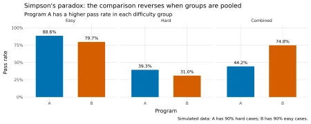
Figure 1: Pass rates within difficulty groups and after pooling students.
Why aggregation changes the comparison
Each pooled pass rate is a weighted average of the rates for easy and hard exams. The weights are the shares of a program’s students in each exam category. Because those shares differ sharply between A and B, each program’s subgroup results contribute to its total in a different proportion.
For A, one tenth of the students take the easy exam and nine tenths take the hard one. Using the observed rates, its weighted result is:
A: (1,000 / 10,000) × (886 / 1,000)
+ (9,000 / 10,000) × (3,536 / 9,000)
= 0.4422 = 44.22%
For B, the weights are reversed: nine tenths take the easy exam and one tenth takes the hard one.
B: (9,000 / 10,000) × (7,169 / 9,000)
+ (1,000 / 10,000) × (310 / 1,000)
= 0.7479 = 74.79%
That arithmetic explains the apparent contradiction. A performs better within each difficulty group, but most of its students sit the exam with the lower pass probability. B’s results are dominated by its much larger easy-exam group.
The reversal is built into the design before the random simulation runs. Apply the specified probabilities directly, and A’s expected pass rate is 45%: 10% of its students have a 90% pass probability, and 90% have a 40% probability. B’s expected rate is 75%, because 90% have an 80% probability and 10% have a 30% probability. Sampling variation shifts the realized results to 44.22% and 74.79%, but it doesn’t create the reversal.
What adjustment can and can’t tell you
In this setup, difficulty is associated with program membership and with the outcome. It therefore acts as a confounder in the comparison: leaving it out combines program differences with the uneven distribution of exam difficulty. Including difficulty in the model lets the analysis compare programs among students facing exams in the same category.
That doesn’t make subgrouping a universal fix. Whether a variable should be included depends on how the variables relate and on the question being asked. Conditioning on a collider, for example, can introduce bias. A reversal is a prompt to inspect the data structure and assumptions, not a standalone instruction to adjust for every available variable.
For analysts, the useful habit is to inspect both the rates and the group counts before interpreting a pooled comparison. In this example, the counts reveal why the aggregate favors B; the within-group rates show how that result changes once exam difficulty is accounted for. A model can make the adjustment explicit, but sound interpretation still depends on understanding how the groups were formed.
The article was first published on R on Zhenguo Zhang's Blog and contributed to R-bloggers. Readers can report an issue, learn about sharing a blog post, or visit R-Posts. Zhang’s Python setup uses plotnine; the source also links to instructions for R, learning R, and R and data science jobs. Readers can comment on the original post or continue to the R-bloggers version.
===