Bitcoin Price Forecasting Combines Neural Networks with GJR-GARCH Volatility Estimates

Price forecasts for Bitcoin that offer only a single number leave out half the story: how uncertain that number is. That gap matters most when volatility changes sharply. The article’s approach pairs a neural network’s return forecast with an econometric model that adjusts the forecast range as market risk changes.

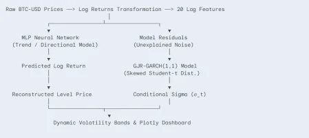
The pipeline combines a Multi-Layer Perceptron built with brulee and tidymodels with a GJR-GARCH model from rugarch. The MLP estimates the expected direction of returns; GJR-GARCH models the volatility around that estimate. It’s a useful division of labor, though the method still depends on assumptions about the return distribution and how well those models fit Bitcoin.

The pipeline starts with returns

Rather than predict Bitcoin’s raw price, the system models log returns and then rebuilds the price path. This helps address the non-stationarity of price levels, which can make direct price modeling unreliable. For price \(P_t\), the return is:

At prediction time, the estimated return is converted back into a price using the previous price:

The architecture is organized around that sequence: forecast returns first, then reconstruct prices and attach a volatility-aware range.

Separate the expected return from the risk

The MLP uses two layers with 32 and 16 units, initialized through tidymodels. It receives 20 days of lagged log returns to learn short- and medium-term autocorrelation. A recipes workflow handles normalization and removes zero-variance predictors, with the stated aim of preventing data leakage.

But a return estimate alone doesn’t describe the clustering of market turbulence: volatile periods often follow volatile periods, while calmer stretches tend to persist too. The pipeline therefore fits GJR-GARCH(1,1) to the MLP’s training residuals, where \(\epsilon_t = r_t - \hat{r}_t\), to estimate conditional variance:

The extra indicator term is the reason to use GJR-GARCH instead of standard GARCH: it allows negative shocks to affect volatility differently from positive ones. The article describes that asymmetry as a feature of crypto markets, where price drops can trigger more panic than equivalent rallies. The model uses one lag for both the ARCH and GARCH terms; the stated rationale is that this captures most volatility persistence without overfitting.

For the return distribution, the implementation specifies skewed Student-t (sstd) to account for heavy tails and asymmetry in Bitcoin returns. It also selects solver = "hybrid" in rugarch, combining optimization methods to help the fit converge with those distribution parameters.

The resulting volatility estimate sets dynamic price bounds around the reconstructed forecast:

Quiet conditions narrow the interval; turbulent ones widen it. That makes the range more responsive than a fixed-width band, though the equations alone don’t establish how well the bounds perform in practice.

Implementation

The article proceeds to a self-contained R script using tidymodels, brulee, rugarch, and plotly to implement the full forecasting pipeline.

[This article was first published on DataGeeek, and kindly contributed to R-bloggers]. (You can report issue about the content on this page here)

Want to share your content on R-bloggers? click here if you have a blog, or here if you don't.

Conclusion

The useful idea here is the division of labor: a neural network forecasts Bitcoin log returns, while a GJR-GARCH model estimates how uncertain those forecasts are over the next 10 days. That pairing can make a forecast’s risk range respond to changing volatility instead of staying fixed.

But the code demonstrates a method, not evidence that it beats a simpler forecast. The accuracy table compares the MLP with a naive model, yet the fragment provides no results. And the plotted bands are derived from residual volatility; they shouldn’t be read as guaranteed 95% coverage. If you’re considering this for trading decisions, the comparison and the band calibration matter as much as the model design.

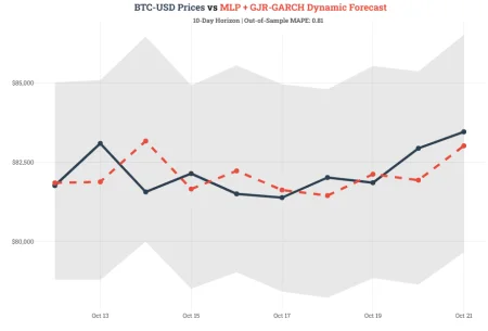
That’s the real promise of the hybrid: a forecast paired with a volatility estimate that can change as market conditions shift. Whether that promise holds up depends on out-of-sample performance and how well the stated bounds match actual outcomes.

To comment on the original article, visit DataGeeek.

R-bloggers.com offers daily email updates about R news and tutorials, including R learning resources. Find or post an R or data science job. To share content on R-bloggers, submit your blog or use R-Posts.

Continue reading: Hybrid Machine Learning & Financial Econometrics: Building Volatility-Aware Dynamic Forecast Bands for Bitcoin