Unlocking Biological Insights through Mathematical Modeling of Variables
Understanding the Relationship Between Biological Variables
In the analysis of biological phenomena, it's essential to grasp how one variable influences another. Take, for instance, a response variable like the weight of an organism. This variable can change based on various predictors, such as time or the amount of fertilizer applied. To encapsulate these associations, scientists utilize mathematical models, which mathematically relate the response to one or more predictors. At its core, any model can be framed as a function where the response is defined in terms of the predictor. This equation takes on a standard form, represented as follows:  Here, **Y** stands for the response variable, **X** denotes the predictor, and **β** signifies a set of parameters, often indicated by Greek or Roman letters, that help define the function's shape. The term **f(…)** represents the specific function itself, outlining the nature of the relationship when plotted in an X-Y graph. Recognizing the significance of mathematical modeling in biology can't be overstated. Researchers must not only familiarize themselves with crucial mathematical functions but also develop the ability to interpret these functions effectively. This means understanding the parameters within them—not just from a mathematical viewpoint, but also in how they relate to biological processes. With this perspective, I've gathered a list of frequently encountered mathematical functions in biology, explaining each of their parameters with a focus on their biological interpretations rather than just their mathematical attributes.Types of Mathematical Functions Encountered in Biology
When plotting these mathematical functions, a common practice is to categorize them based on their shapes on an X-Y graph. This classification isn't arbitrary; it provides insights into the underlying biological dynamics at play. For example, one significant reference in this domain is Ratkowsky's 1990 work, which forms the basis for the following function classifications: 1. **Polynomials** - Straight Line Function - Quadratic Polynomial Function 2. **Concave/Convex Curves (without inflection points)** - Exponential Functions - Asymptotic Functions / Negative Exponential Functions - Power Functions - Logarithmic Functions - Rectangular Hyperbolas 3. **Sigmoidal Curves** - Logistic Functions - Gompertz Functions - Modified Gompertz Functions - Log-Logistic Functions - Weibull Functions (Type 1 and Type 2) 4. **Curves Featuring Maxima/Minima** - Peaked Sigmoidal Functions - Bragg Functions - Lorentz Functions - Beta Functions This list inevitably runs long due to the inclusion of many functions, each with unique attributes and applications. To ease navigation through the material, you can refer to the visual depiction in Figure 1. This figure will help you identify the curve type pertinent to your interests, allowing for quicker access to the relevant discussions.  To clarify symbol meanings, in subsequent discussions, **X** will consistently represent the predictor variable, while **Y** indicates the response variable. Any letters from the Roman alphabet will typically denote model parameters, which together shape the function's overall profile. Understanding these functions and their interpretations is invaluable for anyone working in biological research. By leveraging this mathematical toolkit, scientists can better articulate and quantify the intricate processes they study.Understanding the Logarithmic Function
Logarithmic functions exhibit a distinct linear behavior regarding their parameter,  . The relationship can be illustrated mathematically:
 . Here, the parameter
  significantly impacts the curve's shape. When
  increases, the response
  is the case, an increase in
  represents the response level when
  while maintaining
  (see Fig. 2).
Conversely, dictates the curve's slope, effectively giving the slope value when evaluated at 
D(expression(a + b*log(X)), "X")
b * (1/X)
Altering  results in curves intersecting at
 .</p>
<div class=)
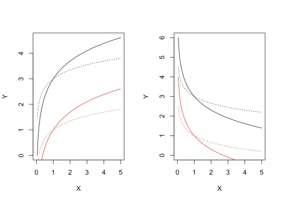
 is fixed to 1 for the solid lines (-1 on the right panel) and 0.5 for the dotted lines (-0.5 in the right panel).
Logarithmic functions find extensive applications in biology. They're frequently employed to model species-area relationships within ecological studies, enzyme kinetics in biochemistry, and various aspects of sensory perception in neurobiology. For practical examples of model fitting, you can refer to this post here.
Conclusions
We've now explored nearly 30 distinct functions that play critical roles in modeling biological processes. Each of these functions has unique characteristics and can be expressed through various parameterizations to fit specific datasets or theoretical frameworks. If you're in the field of biological modeling, consider diving deeper into the work of Miguez et al. (2018); their insights offer valuable perspectives and alternatives that could enhance your modeling efforts. The significance lies not just in the variety of available functions but in how well they can capture the complexities of biological responses. As you apply these models in your own research or practice, stay critical of their statistical properties and adaptability. Remember, the choice of model can significantly affect your results and interpretations. Thanks for sticking with me throughout this discussion! Don’t forget to check out my new book, where I elaborate on these topics and offer practical guidance for applying these functions in real-world scenarios. Prof. Andrea Onofri Department of Agricultural, Food and Environmental Sciences University of Perugia (Italy) Send comments to: andrea.onofri@unipg.it